This article explores the nuanced application of DBSCAN and its fuzzy extension, Fuzzy DBSCAN, in R, showcasing their adeptness at identifying complex and overlapping clusters
Introduction
DBSCAN, also known as Density Based Spatial Clustering of Applications with Noise, stands out as a renowned method in density-based clustering, particularly valued in spatial data mining due to its knack for identifying groups with varying shapes and uniform local density patterns within the feature space. Its effectiveness in discerning clusters amidst noise makes it a favored choice, especially when handling extensive datasets.
Despite its strengths, DBSCAN does face limitations, notably in its capacity to distinguish clusters characterized by fluctuating density distributions and partially overlapping boundaries—a common challenge encountered in scientific and real-world datasets.
In this article, we explore a fuzzy extension of the DBSCAN algorithm designed to generate clusters with fuzzy density attributes. While the original DBSCAN relies on precise parameterization involving parameters like \(minPts\) and \(\epsilon\) to delineate densely populated regions, such rigid values may not always be optimal across all dataset regions. The Fuzzy DBSCAN introduces flexible constraints to define fuzzy cores and borders, offering a nuanced approach to cluster analysis.
Clustering Analysis
Data Preparation
We use several R packages are essential for our clustering analysis: ndefinedfpc, dbscan, fclust, cluster, ggplot2, ppclust, factoextra, and FuzzyDBScan. Each package plays a unique role—from implementing specific clustering algorithms like DBSCAN and fuzzy C-means, to visualizing the results with ggplot2 and fviz_cluster() from the factoextra
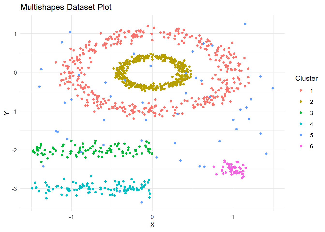
Our analysis utilizes the multishapes dataset, which is a synthetic dataset comprising various geometric shapes. This dataset is particularly suitable for our demonstration because it contains clusters of different shapes and densities, challenging the clustering algorithms to identify these varied patterns.
Code
library(fpc)library(dbscan)library(fclust)library(cluster)library(ggplot2)library(ppclust)library(factoextra)library(FuzzyDBScan)data("multishapes")df <- multishapes[, 1:2]ggplot(multishapes, aes(x = x, y = y, color =as.factor(shape))) +geom_point() +labs(title ="Multishapes Dataset Plot", x ="X", y ="Y", color ="Cluster") +theme_minimal()
It is clear from the plot that there are distinct clusters but with varying density distributions i.e. some clusters are more dense than others. The cluster in yellow forms a dense, ring-like shape in the center, indicative of a well-defined structure. Below that, we see a less dense green cluster stretching horizontally, and a similarly less dense cyan cluster at the bottom. The red and blue clusters appear to be scattered more randomly, which may suggest a different type of grouping or a higher level of noise within these clusters. Finally, the magenta points seem to form a small, separate cluster, likely indicative of a distinct grouping.
K Means Clustering
Let’s start our clustering analysis by using the K Means clustering algorithm.
sil =silhouette(km.res$cluster, dist(df))paste('Silhouette Score: ',round(mean(sil[,'sil_width']),3))
[1] "Silhouette Score: 0.397"
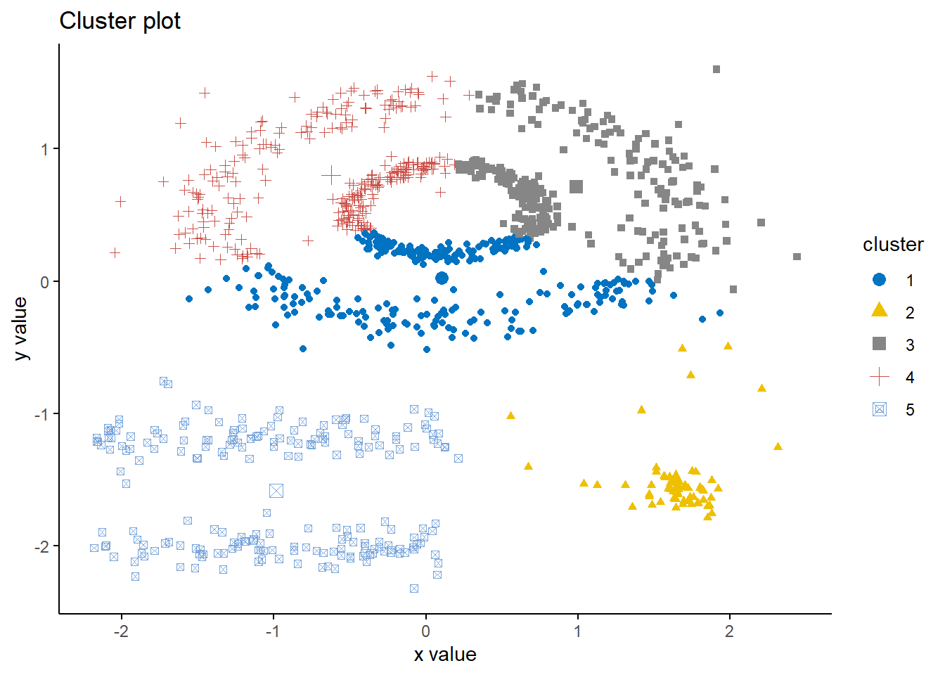
While K-means successfully identifies distinct clusters, it struggles with non-spherical data distributions, as evidenced by the central circular cluster being fragmented into four parts.
A silhouette score of 0.39 indicates moderate separation between clusters. This score ranges from -1 to 1, where a value close to 1 implies that the data points are very clearly matched to their own cluster and poorly matched to neighboring clusters. In contrast, a score close to -1 suggests incorrect cluster assignments. A score around 0 indicates overlapping clusters.
DBSCAN Clustering
The DBSCAN algorithm needs two numeric input parameters, \(MinPts\) i.e. the neighborhood density and \(\epsilon\) i.e. the distance to define local neighborhood size, which together define the desired local density of the generated clusters.
Code
set.seed(2023)db <-dbscan(df, eps =0.15, MinPts =5)fviz_cluster(db, data = df, stand =FALSE, ellipse =FALSE, show.clust.cent = T,geom ="point",palette ="jco", ggtheme =theme_classic())
Code
sil =silhouette(db$cluster, dist(df))paste('Silhouette Score: ',round(mean(sil[,'sil_width']),3))
[1] "Silhouette Score: 0.24"
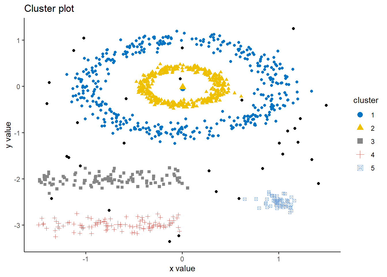
The DBSCAN algorithm demonstrates its strength in handling non-spherical cluster shapes, outperforming K-means in this regard by accurately identifying distinct, non-circular clusters within the data. Moreover, it effectively distinguishes outliers, represented by the black points, which are not encompassed by any cluster due to their sparse distribution. These outliers signify the noise within the dataset that DBSCAN has aptly separated from the more densely packed data points, underscoring its robustness in dealing with real-world data complexities.
However, the silhouette score of 0.24 is pretty low, indicating that the clusters are not as distinct from each other as one might hope.
Determining Optimal\(\epsilon\)
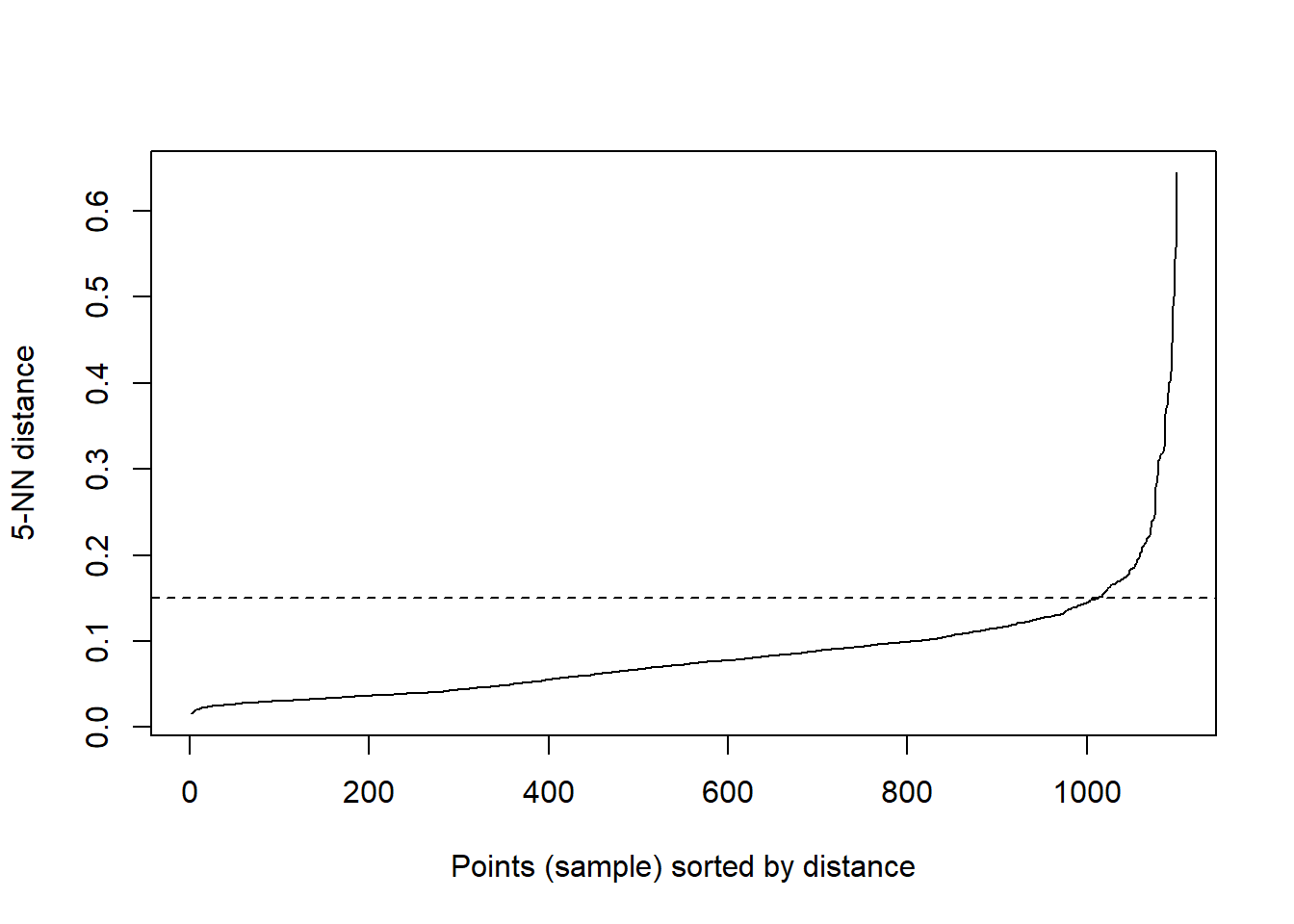
To determine the optimal value for \(\epsilon\), we use a KNN-Distance Plot. It shows the distance to k-nearest neighbor for each point in dataset, sorted in ascending order. The x-axis - represents points in our dataset sorted by distance to their k-th nearest neighbor. We look for an elbow in the graph, i.e. a point where graph changes sharply. This sharp change indicates that we are moving form a dense region (points are close to each other, distance is low) to a sparse one (points are far away).
Code
kNNdistplot(df, k =5)abline(h =0.15, lty =2)
According to this plot \(\epsilon\) = 0.15 seems to be an optimal value.
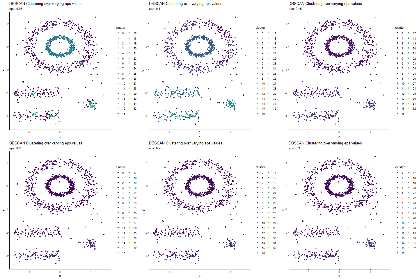
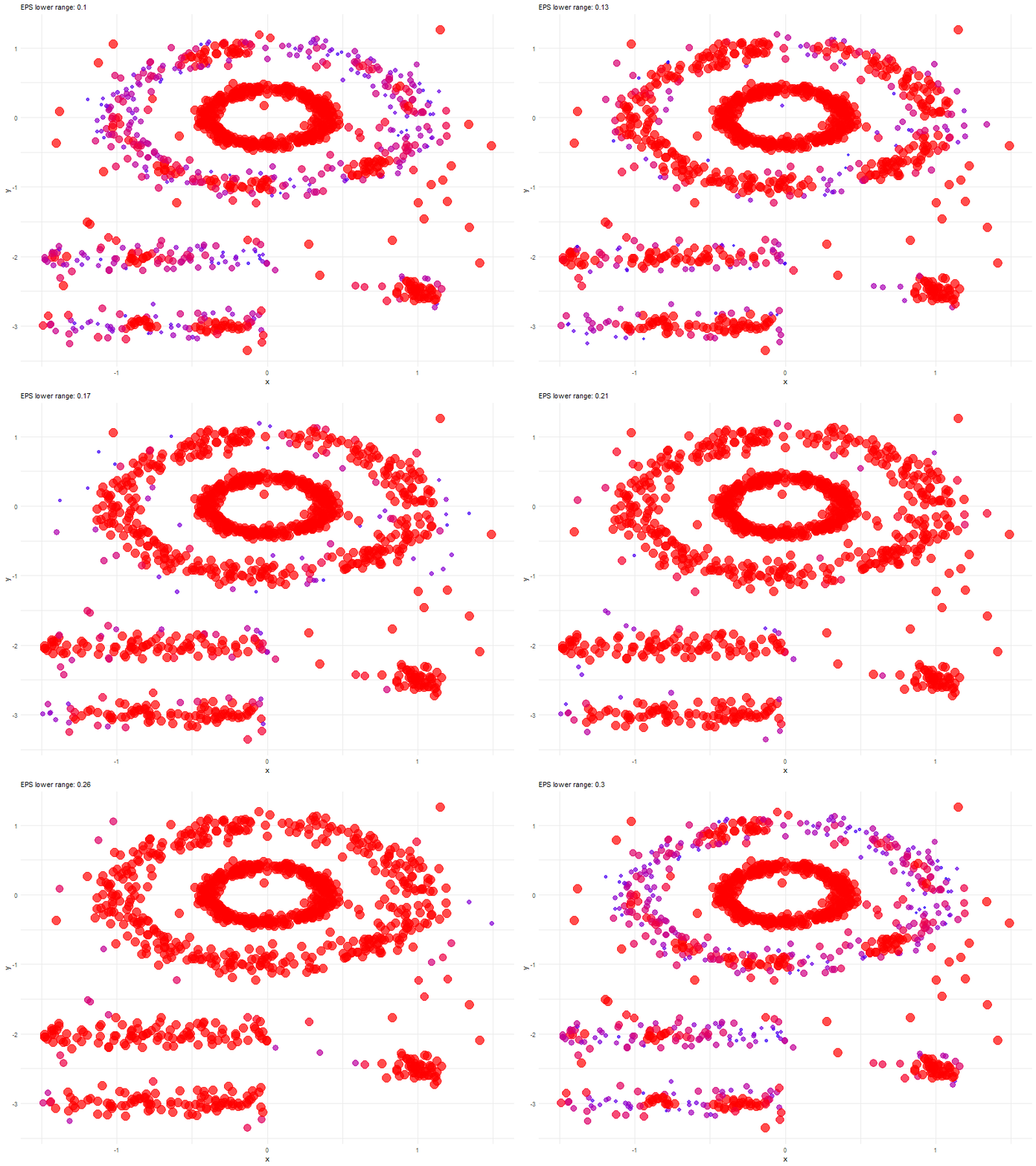
Animated Graph (coded in R) to show changes as we update epsilon
Fuzzy C-Means
Let’s perform Fuzzy C-Means Clustering as well, it should provide us with a good basis for comparison. For a deeper understand of Fuzzy C-means refer to my article.
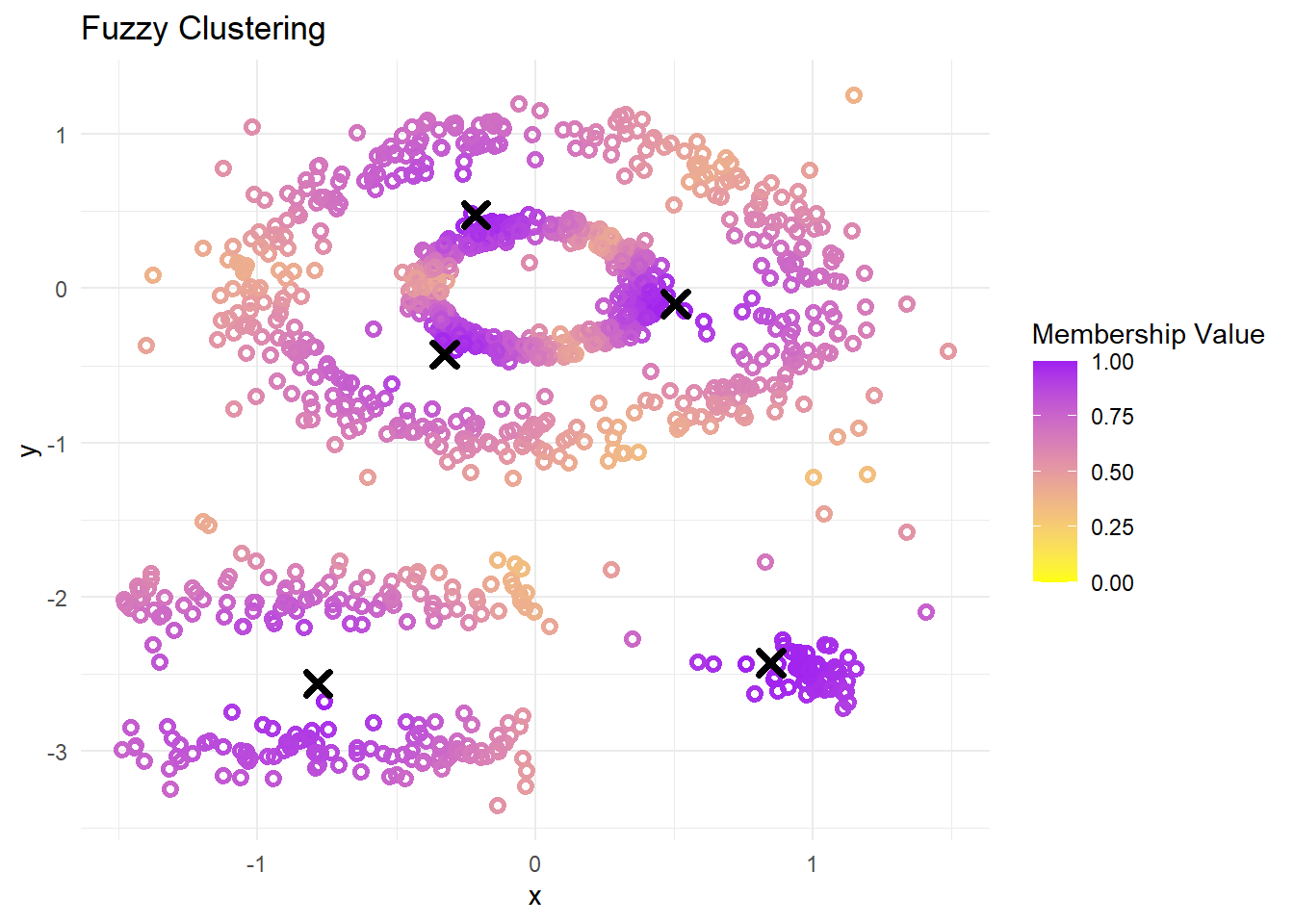
Similar to K-means, we see the Fuzzy c-means does a good job at creating distinct clusters, however, it also does not perform well for non-spherical data distributions. We can see the cluster centers identify do not make sense in the context and structure of the data we have at our disposal.
The Fuzzy Silhouette Score of 0.67 (pretty close to 1) indicates good clustering. Partition Coefficient of 0.57 & Partition Entropy 0.8 indicates that there is moderate cluster overlap, as values closer to 1 would indicate clear, distinct clusters. The partition entropy value, approaching 1, further confirms the presence of some uncertainty in the data points’ cluster memberships.
Fuzzy DBSCAN
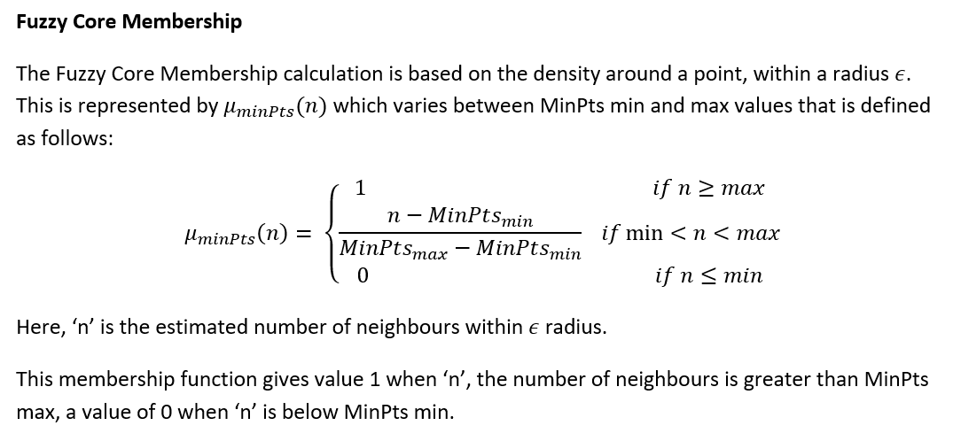
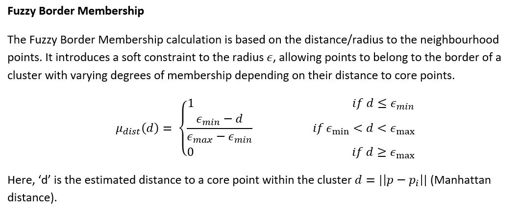
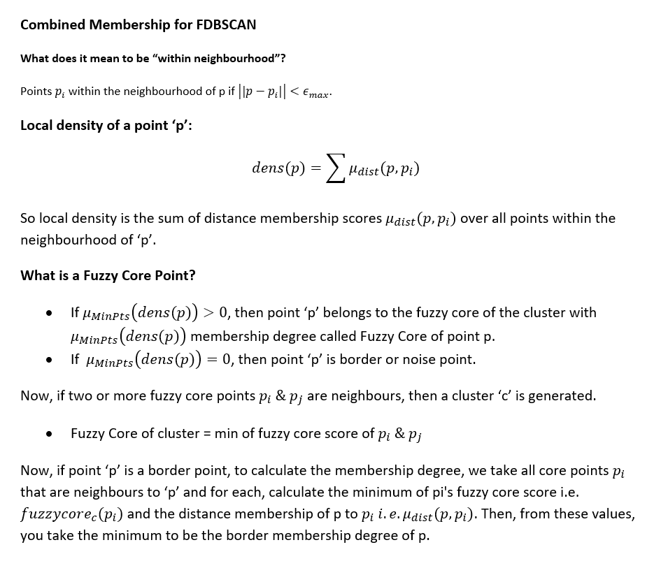
Before delving into its implementation in R, let’s explore the mathematical underpinnings of determining Fuzzy memberships for the clustering algorithm.
Now, let’s proceed with implementing the Fuzzy DBSCAN algorithm. We will utilize the new method to initialize and execute the algorithm. The process involves specifying the dataset along with the values for both parameters.
To implement the Fuzzy Core DBSCAN version, we only specify a range of values for MinPts. Conversely, to implement the Fuzzy Border DBSCAN version, we solely specify a range of values for eps. Supplying ranges for both parameters allows us to implement the complete Fuzzy DBSCAN algorithm.
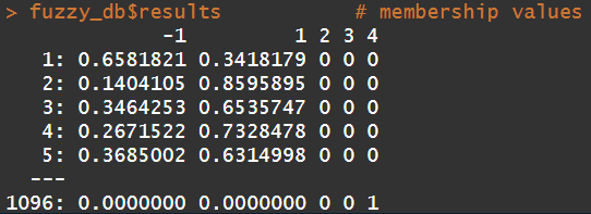
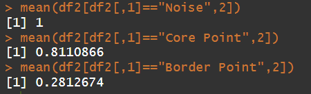
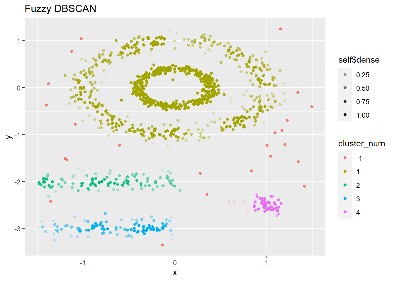
head(fuzzy_db$results, 3) # membership values unique(fuzzy_db$point_def) # category -> noise (-1), core, border pointfuzzy_db$dense # density as a function of nearby neighbours unique(fuzzy_db$clusters) # crisp clusters assignment based on max membershipdf2 =data.frame(fuzzy_db$point_def, fuzzy_db$dense)mean(df2[df2[,1]=="Noise",2]) # average 1 (this is how the algorithm is defined)mean(df2[df2[,1]=="Core Point",2]) # average 0.81 - higher value indicating presence of alot of neighboursmean(df2[df2[,1]=="Border Point",2]) # average 0.28 - lower values
Let’s look at some intermediate results. Firstly we have fuzzy_db$results giving us the Membership values for respective clusters. Cluster -1 membership values are indicative of that data point being a potential outlier.
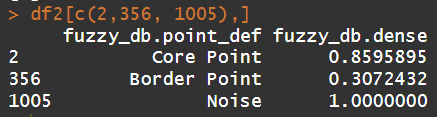
The unique(fuzzy_db$point_def) code returns us the different categories the algorithm divides the data points namely, “Core Point”, “Border Point” and “Noise”. The fuzzy_db$dense code returns us the density values for each data point. Let’s look at these values in the context of their category.
Based on the above results, we can see that the Noise Points have an average density of 1. On analyzing the back-end code of the package, we understand that this is a placeholder value to indicate Noise Points. Looking at the Core and Border Point Densities, we understand the the Core Points have a high density value while the Border Points have low density - accordingly indicative of the number of neighboring points.
Based on these results, the Fuzzy DBSCAN algorithm has effectively grouped the data with a balance between the definition of clusters and the flexibility of fuzzy membership. The clusters are distinct, as indicated by the high partition coefficient of 0.8, and low partition entropy of 0.2, yet there is some degree of uncertainty or overlap among the clusters, as the silhouette score of 0.55 is moderate. Fine-tuning the Fuzzy DBSCAN parameters could potentially yield clusters with sharper definitions.
Before we conclude, here is an animated graph (coded in R) showing changes as we play around with epsilon values.
Conclusion
This article is part of a comprehensive series on Fuzzy Logic and Systems using R, laying the groundwork for understanding advanced concepts and applications in this field.
For further exploration, you can access other articles in this series:
YouTube Video - Clustering with DBSCAN, Clearly Explained!!! by StatQuest with Josh Starmer(link)
Visualizing DBSCAN clustering website by Naftali Harris (link)
These resources offer further insights and practical applications for those interested in advancing their understanding of Fuzzy Logic and its implementations in R.