In this article, we delve into the realm of Fuzzy K Nearest Neighbor (FKNN) and its application in predictive modeling, particularly focusing on the diagnosis of diabetes. We will implement FKNN in R, comparing its performance with the traditional crisp KNN algorithm on a diabetes dataset obtained from Kaggle.
Introduction
Fuzzy logic offers a nuanced approach to decision-making in machine learning, particularly useful when dealing with uncertainty and imprecision in data. Fuzzy K Nearest Neighbor (FKNN) extends the conventional KNN algorithm by incorporating fuzzy membership assignments, providing more nuanced class predictions. In this article, we explore the application of FKNN in the domain of healthcare, specifically in predicting diabetes outcomes based on patient data.
Diabetes Data
For our analysis, we use a comprehensive dataset of diabetes patients sourced from Kaggle. The dataset contains vital patient attributes such as Age, BMI, Blood Pressure, Glucose Level, Insulin Level, Number of pregnancies, and skin thickness. Additionally, it includes the Diabetes Pedigree Function, a metric indicating genetic predisposition to diabetes, along with the binary outcome variable indicating diabetes diagnosis.
Exploratory Data Analysis
Code
library(tidyverse)library(ggplot2)library(class)library(caret)df =read.csv('diabetes.csv')# str(df) # outcome is numericdf$Outcome =as.factor(df$Outcome)summary(df)
  Pregnancies        Glucose      BloodPressure   SkinThickness
 Min.   : 0.000   Min.   :  0.0   Min.   :  0.0   Min.   : 0.00
 1st Qu.: 1.000   1st Qu.: 99.0   1st Qu.: 62.0   1st Qu.: 0.00
 Median : 3.000   Median :117.0   Median : 72.0   Median :23.00
 Mean   : 3.849   Mean   :120.9   Mean   : 69.1   Mean   :20.52
 3rd Qu.: 6.000   3rd Qu.:140.5   3rd Qu.: 80.0   3rd Qu.:32.00
 Max.   :17.000   Max.   :199.0   Max.   :122.0   Max.   :99.00
    Insulin           BMI        DiabetesPedigreeFunction      Age
 Min.   :  0.0   Min.   : 0.00   Min.   :0.0780           Min.   :21.00
 1st Qu.:  0.0   1st Qu.:27.30   1st Qu.:0.2435           1st Qu.:24.00
 Median : 32.0   Median :32.00   Median :0.3740           Median :29.00
 Mean   : 79.9   Mean   :31.99   Mean   :0.4721           Mean   :33.25
 3rd Qu.:127.5   3rd Qu.:36.60   3rd Qu.:0.6265           3rd Qu.:41.00
 Max.   :846.0   Max.   :67.10   Max.   :2.4200           Max.   :81.00
 Outcome
 0:499
 1:268
Code
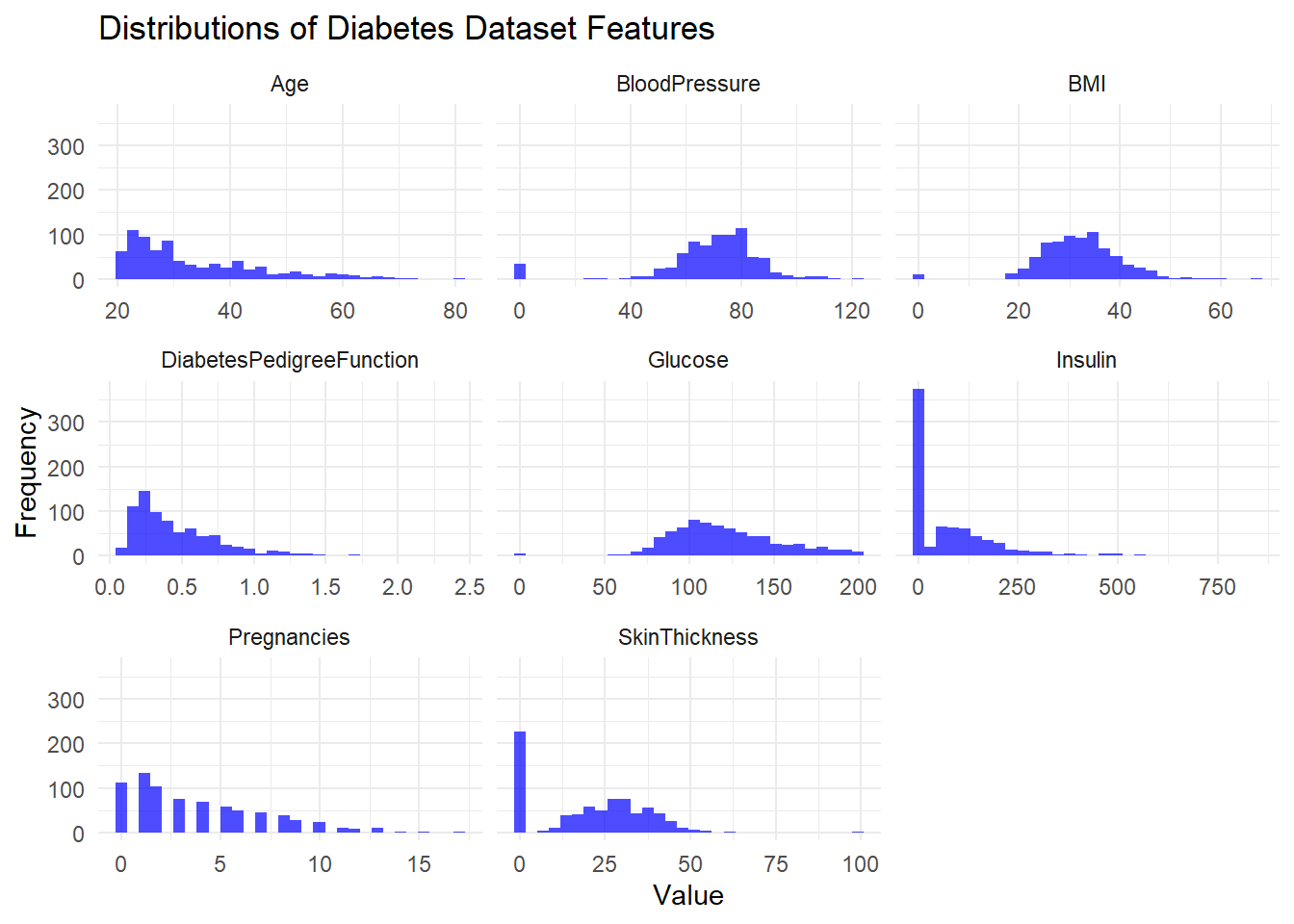
df %>%gather(key ="variable", value ="value", -Outcome) %>%ggplot(aes(x = value)) +geom_histogram(bins =30, fill ="blue", alpha =0.7) +facet_wrap(~variable, scales ='free_x') +theme_minimal() +labs(title ="Distributions of Diabetes Dataset Features", x ="Value", y ="Frequency")
Our dataset unveils captivating insights into the distribution of each variable:
Age: The age distribution skews towards a predominantly young population.
Blood Pressure: Exhibiting a normal distribution, blood pressure spans a diverse range across the dataset.
BMI (Body Mass Index): BMI distribution skews slightly to the right, suggesting a higher prevalence of elevated BMIs and potentially increased chances of diabetes among individuals with higher BMI values.
Diabetes Pedigree Function (DPF): The distribution of DPF, representing genetic influence for diabetes, skews to the right. It’s noteworthy that most individuals possess lower genetic predisposition scores.
Glucose: Arguably the most crucial predictor, the distribution of glucose levels appears to be roughly normally distributed, albeit with a potential right skew. Elevated glucose levels correlate with a higher likelihood of diabetes.
Insulin: Highly right-skewed, the distribution of insulin levels indicates a prevalence of lower values. Extreme high values could potentially denote outliers or erroneous data entries.
Pregnancies: This variable exhibits a somewhat positively skewed distribution, indicating that most women in the dataset have lower pregnancy counts.
Skin Thickness: Skewed to the right, the distribution of skin thickness reveals a peak in lower thickness values. Fewer individuals exhibit higher skinfold thickness, potentially indicating a correlation with diabetes risk factors.
These patterns lay the foundation for our subsequent analysis, providing valuable insights into the dataset’s characteristics and potential predictors of diabetes outcomes.
Code
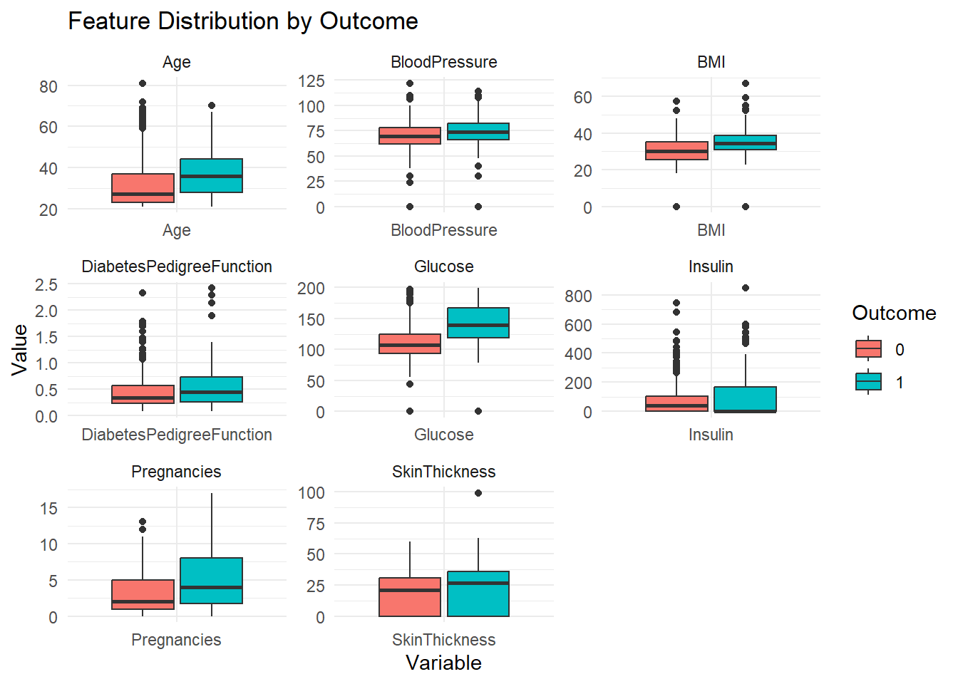
# Boxplots for each feature by Outcome to see the distribution and potential outliersdf %>%gather(key ="variable", value ="value", -Outcome) %>%ggplot(aes(x = variable, y = value, fill =as.factor(Outcome))) +geom_boxplot() +facet_wrap(~variable, scales ='free') +theme_minimal() +labs(title ="Feature Distribution by Outcome", x ="Variable", y ="Value") +scale_fill_discrete(name ="Outcome")
Interpreting the insights gleaned from the boxplots, we observe:
Age: The median age tends to be higher among individuals with diabetes, suggesting a correlation between older age and increased diabetes risk.
Blood Pressure (BP): Higher blood pressure values are associated with a higher likelihood of diabetes diagnosis. This relationship underscores the importance of monitoring blood pressure as a potential risk factor.
BMI (Body Mass Index): Individuals with higher BMI values exhibit an elevated likelihood of diabetes. This finding underscores the significance of maintaining a healthy BMI to mitigate diabetes risk.
Glucose: Elevated glucose levels correspond to a higher probability of diabetes diagnosis. This observation reinforces the critical role of glucose monitoring in diabetes prevention and management.
Based on the compelling associations observed in the boxplots, we opt to focus our analysis on age, blood pressure, BMI, and glucose level as key predictors of diabetes outcomes.
K-Nearest Neighbor (KNN) is a straightforward yet powerful supervised machine learning algorithm used for both classification and regression tasks.
Algorithm Overview:
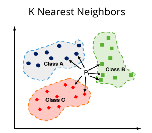
Initialization: We begin by selecting a point (Pt) for which we aim to find its nearest neighbors.
Distance Calculation: Using distance measures such as Euclidean or Manhattan, we compute the distance between the selected point (Pt) and all other data points in the dataset.
Sorting: The calculated distances are then sorted in increasing order, ensuring that the closest neighbors are positioned first.
Assignment:
For classification tasks, we select the ‘k’ closest distances and determine the class that occurs most frequently among these neighbors. This class is then assigned to the selected point (Pt).
In regression tasks, we take the average of the ‘k’ nearest neighbors’ values and assign this average value to the selected point (Pt).
Hyper-parameter ‘k’ Selection: Choosing the appropriate value for ‘k’ is crucial in KNN. A small value of ‘k’ may lead to high variance and low bias, potentially resulting in overfitting. Conversely, a large ‘k’ value may introduce high bias and low variance, indicative of underfitting. Achieving the right balance is essential for optimal model performance.
Now, let’s execute the KNN algorithm in R. First, we ensure that we have appropriate training and test datasets available. Then, we proceed with cross-validation to train the KNN model, selecting the optimal value for the hyper-parameter k using the caret library.
Code
set.seed(123) index <-createDataPartition(df$Outcome, p =0.8, list =FALSE)train_data <- df[index, ]test_data <- df[-index, ]# Scale only the continuous featurestrain_data_scaled <-scale(train_data[,-ncol(train_data)])test_data_scaled <-scale(test_data[,-ncol(test_data)], center =attr(train_data_scaled, "scaled:center"), scale =attr(train_data_scaled, "scaled:scale"))# Convert scaled data back to data.frames and include the Outcome variabletrain_data_scaled <-as.data.frame(train_data_scaled)train_data_scaled$Outcome <- train_data$Outcometest_data_scaled <-as.data.frame(test_data_scaled)test_data_scaled$Outcome <- test_data$Outcometune_result <-train(Outcome ~ ., data = train_data_scaled, method ="knn",trControl =trainControl(method ="cv", number =10),preProcess =c("center", "scale"), tuneLength =10)best_k <- tune_result$bestTune$kknn_model <-knn(train = train_data_scaled[, -ncol(train_data_scaled)], test = test_data_scaled[, -ncol(test_data_scaled)], cl = train_data_scaled$Outcome, k = best_k)# Evaluate model performanceconfusionMatrix(knn_model, test_data$Outcome)
Confusion Matrix and Statistics

          Reference
Prediction  0  1
         0 90 19
         1  9 34

               Accuracy : 0.8158
                 95% CI : (0.7449, 0.874)
    No Information Rate : 0.6513
    P-Value [Acc > NIR] : 6.035e-06

                  Kappa : 0.5758

 Mcnemar's Test P-Value : 0.08897

            Sensitivity : 0.9091
            Specificity : 0.6415
         Pos Pred Value : 0.8257
         Neg Pred Value : 0.7907
             Prevalence : 0.6513
         Detection Rate : 0.5921
   Detection Prevalence : 0.7171
      Balanced Accuracy : 0.7753

       'Positive' Class : 0
Fuzzy KNN
The Fuzzy K Nearest Neighbor (FKNN) algorithm introduces a novel approach to classification by assigning class memberships to our data point Pt rather than rigidly assigning it to a specific class. This paradigm shift enhances the traditional KNN method in two crucial ways:
Fuzzy Membership Assignment: Instead of assigning a data point to a single class, FKNN computes membership values indicating the degree of belongingness to different classes. This nuanced approach enables FKNN to capture the uncertainty inherent in classification tasks, providing a more comprehensive representation of the data.
Distance Weighting: In FKNN, the influence of neighboring points on membership values is inversely related to their distance from the target point. Closer neighbors exert a stronger influence, while farther ones contribute less. This distance-weighting mechanism, governed by a tunable parameter ‘m’, ensures that FKNN prioritizes nearby neighbors, thereby mitigating the risk of misclassifying points in overlapping regions.
Traditional KNN algorithms treat all neighbors equally, potentially leading to misclassifications in regions with overlapping class boundaries. Moreover, the binary class assignments offered by conventional KNN lack the granularity to convey confidence levels in classification outcomes.
FKNN addresses these limitations by leveraging membership degrees, which serve as a level of assurance for classification results. Higher membership values indicate stronger associations with specific classes, enhancing the interpretability and reliability of the classification process.
Furthermore, FKNN’s flexibility shines through its ability to tune the hyper-parameter ‘m’ according to the problem domain’s specific characteristics. This adaptability empowers practitioners to tailor FKNN to diverse datasets and classification challenges, enhancing its applicability across a wide range of scenarios.
In summary, FKNN offers a sophisticated yet intuitive framework for classification tasks, leveraging fuzzy logic principles to improve accuracy, interpretability, and adaptability in comparison to traditional KNN approaches.
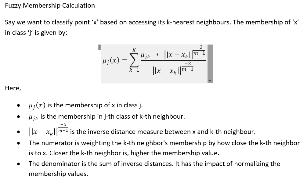
Fuzzy Membership Calculation
Understanding the role of ‘M’
The hyper-parameter ‘m’ plays a pivotal role in shaping the behavior of the Fuzzy K Nearest Neighbor (FKNN) algorithm, influencing how the distances between neighbors are weighted when calculating their contributions to the membership values.
For m = 2: The contributions of each neighbor, specifically the k-th neighbor, are weighted by the reciprocal of their distance from the target point. As a result, closer neighbors exert a stronger influence on the membership values, while farther neighbors have a diminished impact.
As the Value of ‘M’ Increases: With higher values of ‘m’, the distribution of weights among neighbors becomes more even. This leads to a more uniform distribution of influence, where the relative distances of neighbors from the target point have less effect. Consequently, points that are farther away from the target point can also significantly influence the membership values. This property facilitates the creation of smoother and more generalized decision boundaries, making the algorithm robust against high levels of overlap or noisy data.
As the Value of ‘M’ Tends to 1: Conversely, when ‘m’ approaches 1, closer neighbors are heavily weighted, while the number of points contributing to the membership values decreases. This results in an emphasis on immediate neighbors, leading to a classification process that is highly sensitive to the local structure of the data. While this sensitivity enables the model to capture finer details and variations in the data, it also renders the classification results more susceptible to noise and outliers.
In conclusion, the choice of ‘m’ allows practitioners to fine-tune the behavior of the FKNN algorithm based on the specific characteristics of the dataset and the desired level of sensitivity to local structure. By carefully selecting an appropriate value for ‘m’, practitioners can strike a balance between capturing intricate patterns in the data and maintaining robustness against noise and outliers.
R Implementation
Now, let’s proceed with implementing Fuzzy K Nearest Neighbor (FKNN) in R. To facilitate this, we’ll begin by creating a custom function that takes the training and test features and labels as inputs, along with the hyperparameters k and m. While drawing inspiration from an existing R library (Github link), we’ll make a small correction in the function.
# Data preparationtrain_features <-as.matrix(train_data_scaled[, -ncol(train_data_scaled)])train_labels <-model.matrix(~ Outcome -1, data = train_data_scaled)test_features <-as.matrix(test_data_scaled[, -ncol(test_data_scaled)])test_labels <- test_data_scaled$Outcomek <- best_k # This is the best k from your previous KNN modelm <-3fuzzy_knn_predictions <-fknn(train_features, train_labels, test_features, k, m)# class with highest membership valuebinary_predictions <-apply(fuzzy_knn_predictions, 1, which.max) # convert to factorsbinary_predictions <-factor(binary_predictions, labels =levels(df$Outcome))confusionMatrix(binary_predictions, test_labels)
Confusion Matrix and Statistics

          Reference
Prediction  0  1
         0 91 16
         1  8 37

               Accuracy : 0.8421
                 95% CI : (0.7742, 0.8961)
    No Information Rate : 0.6513
    P-Value [Acc > NIR] : 1.266e-07

                  Kappa : 0.6397

 Mcnemar's Test P-Value : 0.153

            Sensitivity : 0.9192
            Specificity : 0.6981
         Pos Pred Value : 0.8505
         Neg Pred Value : 0.8222
             Prevalence : 0.6513
         Detection Rate : 0.5987
   Detection Prevalence : 0.7039
      Balanced Accuracy : 0.8087

       'Positive' Class : 0
Grid Search for Hyperparameter Tuning
To identify the optimal values for the hyperparameters k and m in our Fuzzy K Nearest Neighbor (FKNN) model, we can conduct a grid search. While the following code snippet may not be executed each time the article loads, you can run it locally to perform the grid search and fine-tune the model’s performance.
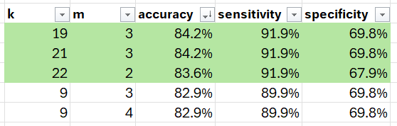
After conducting the grid search to identify the optimal values for the hyperparameters ‘k’ and ‘m’ in our Fuzzy K Nearest Neighbor (FKNN) model, we obtained the following results:
These are the top 5 results. Based on this, we can select top 19 neighbors and m = 3 as our fuzziness parameter.
Conclusion
This article is part of a comprehensive series on Fuzzy Logic and Systems using R, laying the groundwork for understanding advanced concepts and applications in this field.
For further exploration, you can access other articles in this series: