Fuzzy Time Series in R & Python

Abstract

In this article we study and implement Fuzzy Time Series in R.

Introduction

Fuzzy sets and models have the ability to approximate functions along with it, it brings an element of explainability by use of linguistic variables and rules. The idea of Fuzzy Time Series (FTS) is to divide the Universe of Discourse of the time series into intervals/partitions (fuzzy sets), and learn how each area behaves (extracting rules through the time series patterns).

Fig: Overview of Fuzzy Time Series Modelling

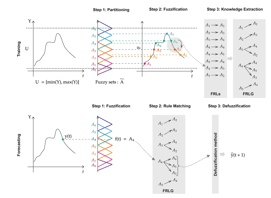
There are two kinds of Fuzzy Time Series \(F_t\) models: time variant and time invariant. If for any time ‘t’, the fuzzy logic relationship \(R_{t, t-1}\) is independent of ‘t’, then \(F_t\) is called a time-invariant fuzzy time series. Otherwise, it is called a time-variant fuzzy time series.

Fuzzy time series models can be divided into two classes, which are called first-order and high-order models. If \(F_t\) is caused by \(F_{t-1}\) only i.e. \(F_{t-1} \rightarrow F_t\), then the first-order forecasting model can be expressed as \(F_t = F_{t-1} \circ R_{t,t-1}\) where \(R_{t,t-1}\) is the fuzzy relationship. In high-order models, \(F_t\) is dependent on more past values.

General Steps of FTS modeling :

1. Define the Universe of Discourse (U).
2. Data Partitioning i.e. dividing U into intervals which represent our fuzzy sets.
3. Fuzzification i.e. representing crisp time series values by fuzzy sets & memberships.
4. Formulation of Fuzzy Logic Relations and Groups
5. Defuzzification & Forecasting.

Enrollment Time Series

We have a time series of historical enrollments of the University of Alabama from 1971 to 1992. First let’s perform some exploratory analysis and then fit an ARIMA model which will be our baseline for evaluating fuzzy models.

library(AnalyzeTS)
library(ggplot2)
library(forecast)
library(Metrics)

data(enrollment)
cat("Range of values:",min(enrollment),'to',max(enrollment))

Range of values: 13055 to 19337

Step 1: Define Universe of Discourse

We start by defining the Universe of Discourse U. We define \(U = [min(X_t)-d_1, max(X_t)+d_2]\) where \(d_1, d_2\) are positive numbers, expanding the range of our time series, creating a security margin for future predictions. Given the range of Enrollments is from 13055 to 19337, let’s take \(d_1 = 55, d_2 = 663\) giving us U = [13000, 20000].

Step 2: Data Partitioning

There are various ways to partition our universe of discourse. The simplest approach is dividing in intervals of equal length. So let’s partition U into seven equal intervals (with a gap of 1000 each) where \(u_1\) = [13000, 14000], \(u_2\) = [14000, 15000] … \(u_7\) = [19000, 20000].

For unequal intervals, we can use (a) Mathematical Models or (b) Soft Computing Techniques. Mathematical models consist of distribution-based, average-based, frequency-density based, ratio-based, entropy-discretisation based models. On the other hand, Soft Computing techniques can be further broken down into two categories; (i) Optimization-based and (ii) Clustering based. Optimization based techniques use Particle Swarm Optimization for example, while clustering techniques like fuzzy c-means or dynamic time wrapping can also be used.

Step 3: Fuzzification

These 7 intervals become our 7 fuzzy sets. We can represent them using linguistic variables like \(A_1\) = not many, \(A_2\) = not too many, \(A_3\) = many, \(A_4\) = many many, \(A_5\) = very many, \(A_6\) = too many, \(A_7\) = too many many.

Step 4: Formulation of Fuzzy Logic Relations and Groups

Next step is to fuzzify our inputs i.e. converting them from crisp numerical values into fuzzy values. Here, we create fuzzy logic relations (FLR) in the form of \(Precedent \rightarrow Consequent\) for example, \(A1 \rightarrow A2\) means the series was in A1 at time ‘t’, will be in A2 are time ‘t+1’. Next, \(A2 \rightarrow A2\) implies it stays in A2 from ‘t+1’ to ‘t+2’.

Now, we can group the FLRs based on the precedents, creating our Fuzzy Logic Rule Groups (FLRGs). For example, we have \(A1 \rightarrow A1, A2\) implying that from A1 we can either stay in \(A_1\) or move to \(A_2\). These rules describe the behavior of our time series and are used to forecast future values.

Step 5: Defuzzification & Forecasting

Lastly, we want to defuzzify and make predictions. For this we can either consider the single max membership, or consider all consecutive max memberships and take average of respective midpoints. Say we have a fuzzy output = [0, 0.5, 1, 1, 1, 0.5]. Since, consecutive max memberships are for sets 3, 4 and 5, we take average of their mid-points. If the fuzzy output was [0, 0, 0, 1, 0, 0], then we take the midpoint of interval represent set 4.

ggtsdisplay(enrollment, smooth = T)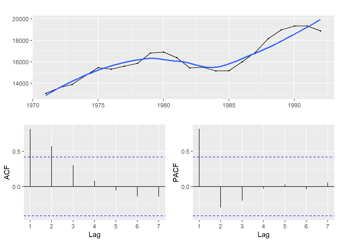

From the graph of the series, we can see that it has an overall upward trend making it non-stationary. The same is reflected in the sample ACF graph.

ARIMA Model

fit = auto.arima(enrollment) # ARIMA(1,1,0)
plot(fit$fitted, main='ARIMA(1,1,0) Model')
points(fit$fitted,cex=0.5)
lines(enrollment, col='red')
points(enrollment, col='red',cex=0.5)
legend('topleft',c('Enrollment','fitted ARIMA(1,1,0)'), 
       col=c('black','red'),lwd=3,bty='n',lty=1)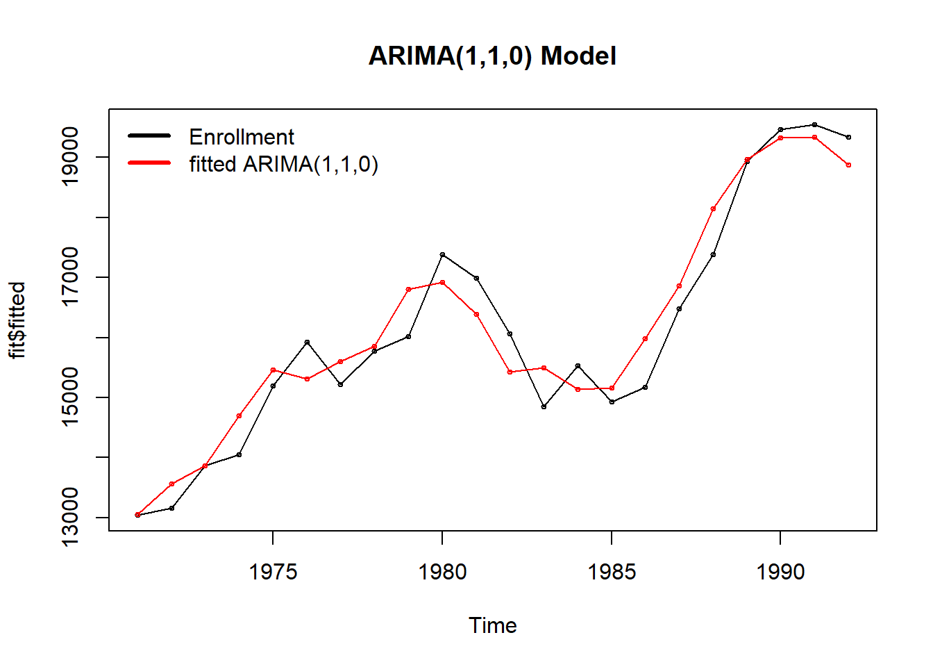

cat("MAPE =",round(100*mape(enrollment, fit$fitted),2),"%")

MAPE = 2.52 %

The fitted ARIMA(1, 1, 0) confirms that the original series is not stationary (order d = 1). The plot above, shows that our ARIMA models does a very decent job at capturing the enrollment time series.

Fuzzy Time Series

The traditional ARIMA models can predict seasonality but fail to forecast problems with linguistic historical data. Furthermore, traditional time series methods requires more history data and data must be normally distributed to get a better forecasting performance. However, there are often not sufficient data in all kinds of time series model, and linguistic expressions are often used to describe daily observations. To deal with these kinds of problems, fuzzy time series is proposed.

The AnalyzeTS package provides us with fuzzy.ts1() & fuzzy.ts2() commands to fit fuzzy time series models Chen (1996), Singh (2008), Heuristic (2001) and Chen-Hsu (2004) and Abbasov-Mamedova, (2004). Here we implement steps 3, 4, 5 all at once. Now let’s divide into understanding some of the fuzzy time series models.

Song-Chissom (1993)

Song and Chissom developed a first-order time invariant model : \(A_i = A_{i=1} \circ R\), where \(A_{i-1}\) is the fuzzy set for enrollment of year \(i-1\), “\(\circ\)” is the min-max composition operator, and \(R\) is the fuzzy relationship matrix.

First, Song and Chissom define operator “x”: \((i, j)^{th}\) element of \(D^T\) x \(B = min(D_i, B_j)\). We evaluate \(R_1 = A^T_1\)x\(A_1\), \(R_2 = A^T_1\)x\(A_2\), …, \(R_9 = A^T_6\)x\(A_6\), \(R_10 = A^T_6\)x\(A_7\). The final fuzzy relation R = \(U_{i=1}^{10} R_i\).

The problem with this model is that it requires large amount of computation to derive fuzzy relations and perform min-max compositions.

Chen (1996)

In 1996, Shyi-Ming Chen proposed a modification to Song-Chissom model by using simplified arithematic operations rather than complicated min-max composition operations.

• Step 1 - Define Universe of Discourse (U)

• Step 2 - Data Partitioning - divide U into intervals of equal length.

• Step 3 - Fuzzification

• Step 4 - Formulation of FLR

• Step 5 - Defuzzification & Forecasting

  Forecasting rule: (a) if there is one fuzzy rule applicable i.e. \(A_i \rightarrow A_j\) then we consider the mid-point of interval in which \(A_j\) belongs. (b) if there are multiple fuzzy rules applicable, then we take average of all midpoints of respective the sets. Let’s take two examples:

  • For year \(1974\rightarrow1975\), we have \(A_2 \rightarrow A_3\) i.e. only one rule, thus, forecast = midpoint of interval of \(A_3\), [15000 16000] i.e. 15500.

  • For year \(1975 \rightarrow 1976\), we have \(A_3 \rightarrow A_3\) and \(A_3\rightarrow A_4\) rules applicable. Thus, forecast = average of midpoints of intervals [15000 16000] and [16000 17000] = 0.5*(15500 + 16500) = 16000.

D1 = 55    
D2 = 663 
n = 7    # number of intervals/ fuzzy sets  

# Chen, 1996 
fit = fuzzy.ts1(ts = enrollment,n = n,D1 = D1,D2 = D2,
                type = "Chen",plot = TRUE, trace = T, grid = T)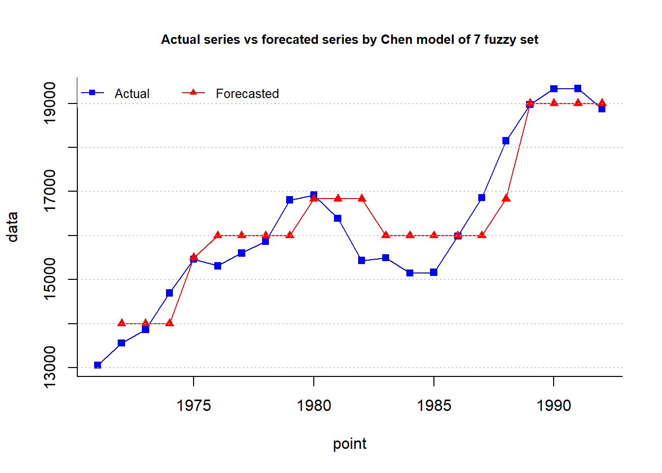 

cat("MAPE =",fit$accuracy[4],"%")

MAPE = 3.11 %

fit$table1

  set   dow    up   mid num
1  A1 13000 14000 13500   3
2  A2 14000 15000 14500   1
3  A3 15000 16000 15500   9
4  A4 16000 17000 16500   4
5  A5 17000 18000 17500   0
6  A6 18000 19000 18500   3
7  A7 19000 20000 19500   2

Table 1 contains information about the fuzzy sets formulated. The first column shows the ‘n’ number of fuzzy sets formed, the interval range and respective mid-points. The last column shows the count of observations in each set.

fit$table2

   point actual relative forecasted
1   1971  13055  A1-x-NA         NA
2   1972  13563  A1<--A1   14000.00
3   1973  13867  A1<--A1   14000.00
4   1974  14696  A2<--A1   14000.00
5   1975  15460  A3<--A2   15500.00
6   1976  15311  A3<--A3   16000.00
7   1977  15603  A3<--A3   16000.00
8   1978  15861  A3<--A3   16000.00
9   1979  16807  A4<--A3   16000.00
10  1980  16919  A4<--A4   16833.33
11  1981  16388  A4<--A4   16833.33
12  1982  15433  A3<--A4   16833.33
13  1983  15497  A3<--A3   16000.00
14  1984  15145  A3<--A3   16000.00
15  1985  15163  A3<--A3   16000.00
16  1986  15984  A3<--A3   16000.00
17  1987  16859  A4<--A3   16000.00
18  1988  18150  A6<--A4   16833.33
19  1989  18970  A6<--A6   19000.00
20  1990  19328  A7<--A6   19000.00
21  1991  19337  A7<--A7   19000.00
22  1992  18876  A6<--A7   19000.00

Table 2 contains information about the fuzzy series showing the actual and forecasted value along with the fuzzy relationship applicable for every value of \(F_t\).

fit$relative.groups

[1] “A1->A1,A2” “A2->A3” “A3->A3,A4” “A4->A3,A4,A6” “A5->NA,”
[6] “A6->A6,A7” “A7->A6,A7”

Relative groups are the Fuzzy Logic Relationship Groups (FLRGs) formed by the algorithm.

library(ggplot2)
plot.my.fuzzy.sets = function(table){
  ggplot(data = table, aes(x=mid))+
  geom_segment(aes(x=dow, xend=mid, y=0, yend=1),color='navy')+
  geom_segment(aes(x=mid, xend=up, y=1, yend=0),color='navy')+
  geom_point(aes(y=0), color='red')+
  geom_text(aes(label = set, y = 0.5), vjust = 0, size = 3) +
  scale_x_continuous(name = "Universe of Discourse") +
  scale_y_continuous(name = "Membership Degree", limits = c(0, 1)) +
  ggtitle("Fuzzy Sets Visualization") +
  theme_minimal()
}
plot.my.fuzzy.sets(fit$table1)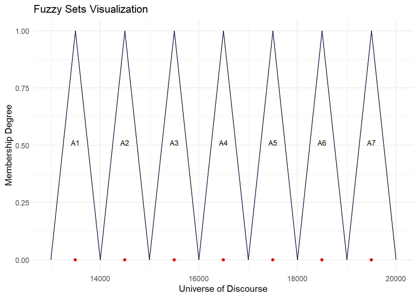

Heuristic (Huarng, 2001)

Heuristic means domain-specific knowledge. In 2001, Kunhuang Huarng modified Chen’s model by integrating heuristic knowledge. Here, the heuristic knowledge ‘h’ shows the increase or decrease in enrollment.

• Step 1 - Define Universe of Discourse (U)

• Step 2 - Data Partitioning - divide U into intervals of equal length.

• Step 3 - Fuzzification

• Step 4 - Formulation of Fuzzy Logic Relationship Groups.

• Step 5 - Formulation of Heuristic Fuzzy Relationship Groups.

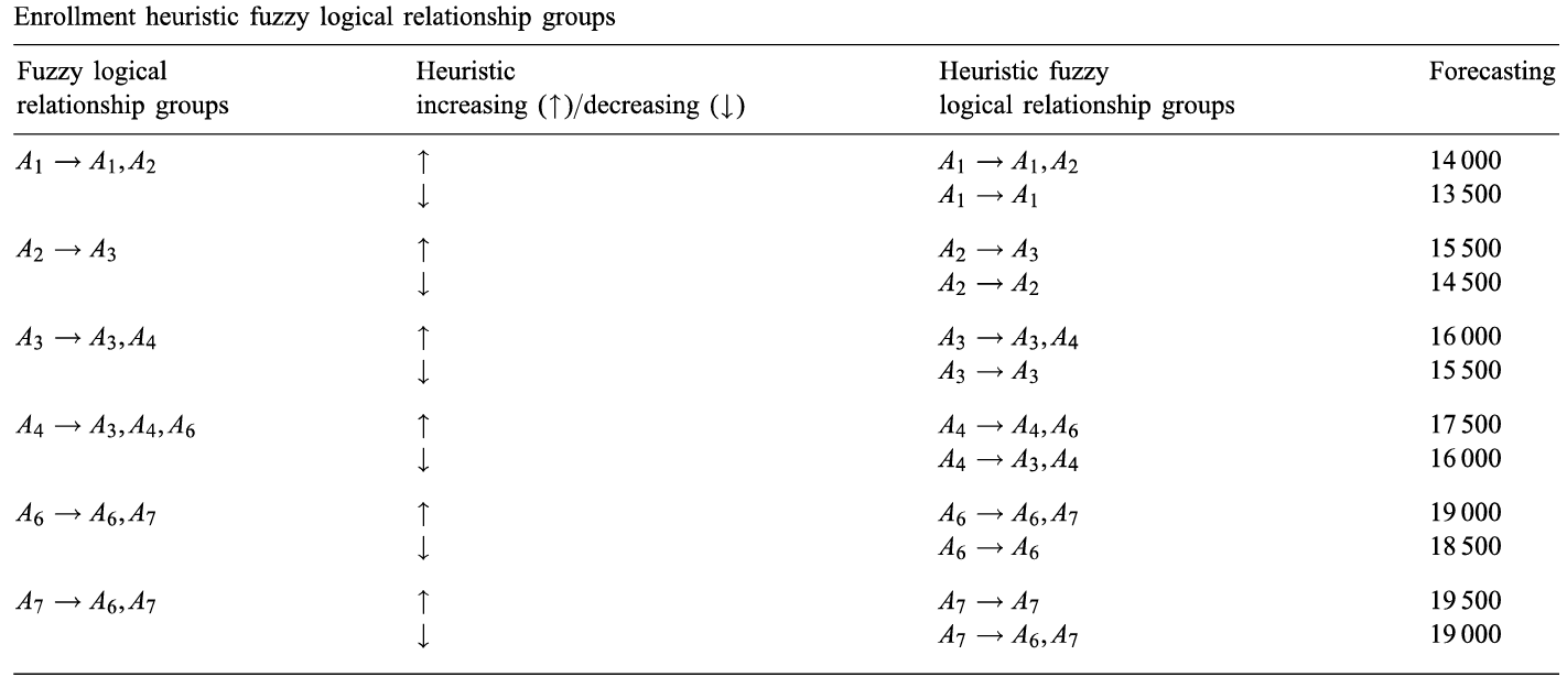
So if heuristic knowledge points upwards, we split \(A_1 \rightarrow A_1, A_2\) into \(A_1 \rightarrow A_1, A_2\) for upwards and \(A_1 \rightarrow A_1\) for downwards.

• Step 6 - Defuzzification & Forecasting

  • For 1975, the actual value for 1974 is 14,696 belonging to \(A_2\) and 1974 \(\rightarrow\) 1975 is given by \(A_2 \rightarrow A_3\). From the table above, suppose the heuristic points upwards. So, forecast is mid point of interval corresponding to \(A_3\) i.e. 15,500.

  • For 1977, the actual value for 1976 is 15,311 belonging to \(A_2\) and 1976 \(\rightarrow\) 1977 is given by \(A_3 \rightarrow A_3\). From the table above, suppose the heuristic points downwards. So, forecast is mid point of interval corresponding to \(A_2\) i.e. 14,500.

  Now the question arises, what is this “heuristics” that we are using? The heuristics are a combination of historical data analysis and domain expertise that capture underlying patterns and volatility of the time series. Suppose we have a stock price time series, we can use various stock-market indexes, inflation rates, interest-rate fluctuations, competing company/industries’ stock price behavior as heuristics to guide whether our series will increase or decrease.

  We can also use changes in the process itself, as heuristics to guide the increase/decrease changes.

  head(cbind(enrollment, 
             diff = c(NA, diff(enrollment, differences = 1))))

  Time Series:
  Start = 1971 
  End = 1976 
  Frequency = 1 
       enrollment diff
  1971      13055   NA
  1972      13563  508
  1973      13867  304
  1974      14696  829
  1975      15460  764
  1976      15311 -149

  Here, if the difference values are positive then we consider upward movement and vice-versa.

  • For example, year 1972, the difference of 508 is positive, so we have upward movement. Respective fuzzy logic relationship is \(A_1 \rightarrow A_1, A_2\) and the upwards movement gives us heuristic relationship of \(A_1 \rightarrow A_1, A_2\). Thus, forecast is average of mid points of intervals corresponding to \(A_1, A_2\) = 14000.

  • For year 1976, the difference of -149 is negative, so we have downward movement. Respective fuzzy logic relationship is \(A_3 \rightarrow A_3, A_4\) and the downwards movement gives us heuristic relationship of \(A_3 \rightarrow A_3\). Thus, forecast is mid point of interval corresponding to \(A_3\) = 15,500.

# Heuristic (Huarng, 2001) 
fit = fuzzy.ts1(ts = enrollment,n = n,D1 = D1,D2 = D2,           
                type="Heuristic",plot=TRUE, trace = T, grid = T)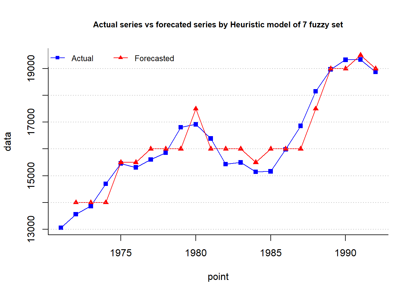 

head(fit$table2) # image above

  point actual relative forecasted
1  1971  13055  A1-x-NA         NA
2  1972  13563  A1<--A1      14000
3  1973  13867  A1<--A1      14000
4  1974  14696  A2<--A1      14000
5  1975  15460  A3<--A2      15500
6  1976  15311  A3<--A3      15500

cat("MAPE =",fit$accuracy[4],"%")

MAPE = 2.445 %

plot.my.fuzzy.sets(fit$table1)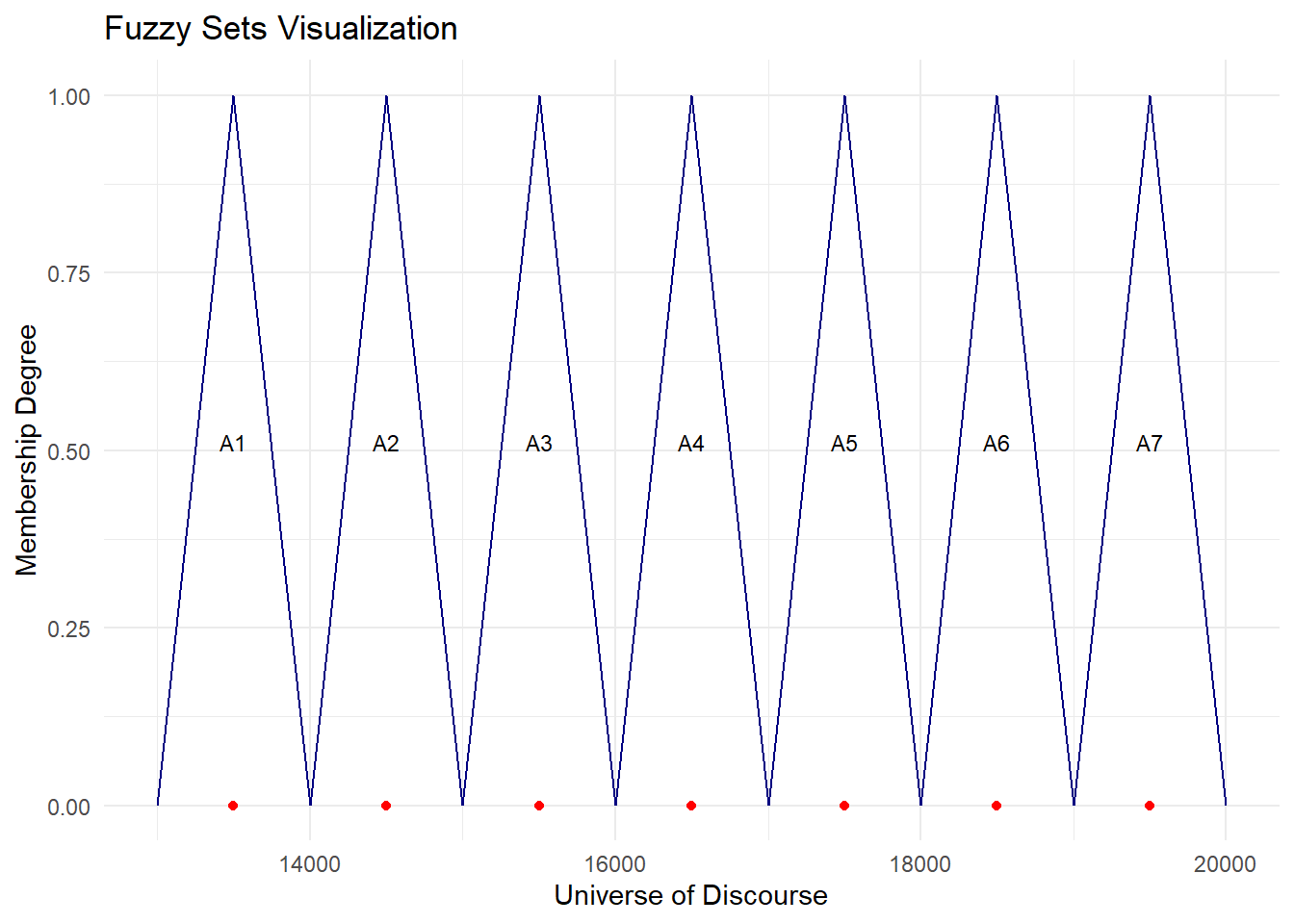

Singh (2008)

In 2008, S.R. Singh introduced a computational method of forecasting based on fuzzy time series to provide improved forecasting results to cope up with the situation containing higher uncertainty due to large fluctuations in consecutive year’s values in the time series data and having no visualization of trend or periodicity. The proposed model is of order three and uses a time variant difference parameter on current state to forecast the next state.

Here we perform all the respective steps similarly, the only difference lies at the defuzzification and forecasting step. The proposed forecasting algorithm is quite complex (refer to research paper).

# Singh, 2008 
fit = fuzzy.ts1(ts = enrollment,n = n,D1 = D1,D2 = D2,                 
                type="Singh",plot=TRUE, trace = T, grid = T)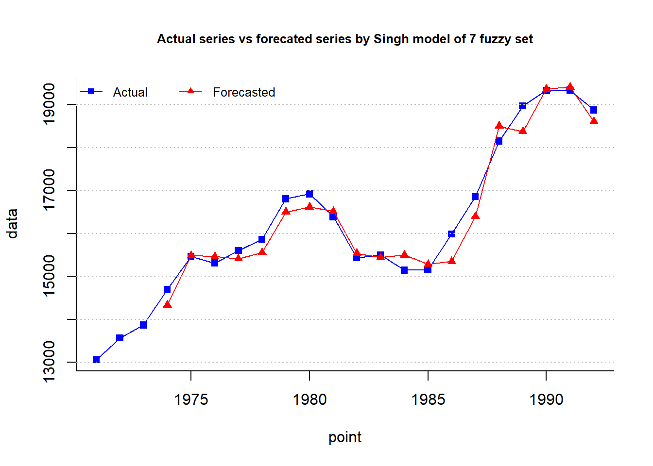 

cat("MAPE =",fit$accuracy[4],"%")

MAPE = 1.531 %

plot.my.fuzzy.sets(fit$table1)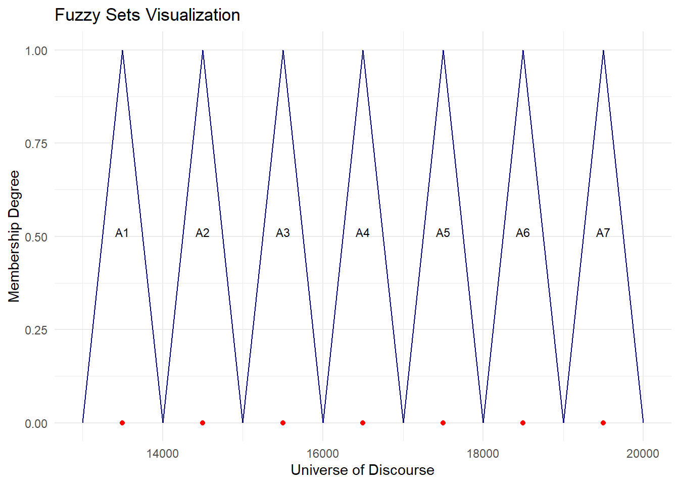

Chen-Hsu (2004)

In 2004, Shyi-Ming Chen and Chia-Ching Hsu proposed a model with the aim to improve forecasting accuracy.

Here we perform all the respective steps similarly, the only difference lies at the defuzzification and forecasting step. The proposed forecasting algorithm involves considering difference of difference of three past year values of the series, this helps evaluate the trend in the series. If the trend is upwards, we consider the 75th percentile of the respective interval, trend is downwards then 25th otherwise 50th percentile.

• For example, \(trend = |(X_{1975}-X_{1974})-(X_{1974}-X_{1973})| = 65\). Now we calculate (a) 2 x trend + \(X_{1975}\) = 15590 and (b) 0.5 x trend + \(X_{1975}\) = 15492.5. Now we consider the interval of \(X_{1975} = 15460\) i.e. [15250, 15500].

  • If (a) lies in this interval, we consider the 75th percentile of the interval as the forecast, as the trend is upwards.

  • If (b) lies in this interval, we consider 25th percentile of the interval as the forecast, as the trend is downwards.

  • If neither is the case, we consider the middle value of the interval.

• So here we take 25th percentile of interval = 15312.5 which is our forecasted value.

• The ChenHsu.bin() command allows us to divide the fuzzy sets further if we want. For now, we specify n.subset = rep(1, n) i.e. divide the existing 7 intervals into 1 part only (i.e. no division). If we specify n.subset = (1,2,3,4,1,1,1), then we divide 2nd interval into 2 equal parts, 3rd into 3, 4th in 4 equal parts and remaining intervals stay the same. We will use this in the section below where we explore alternatives of FTS modeling.

  # Chen-Hsu, 2004 
  A = fuzzy.ts1(enrollment,n = n,type = "Chen-Hsu",plot = 1) 
  
  B = ChenHsu.bin(A$table1, n.subset = rep(1, n)) 
  
  fit.chen.hsu = fuzzy.ts1(enrollment, type = 'Chen-Hsu', 
                           bin = B, plot = 1, trace = 1)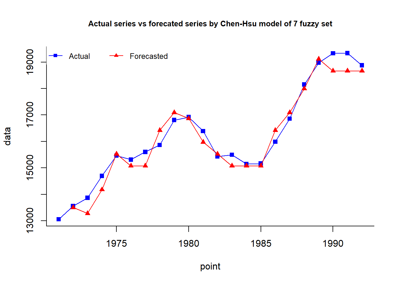 

  

  cat("MAPE =",fit.chen.hsu$accuracy[4],"%")

  MAPE = 1.893 %

  A

  $type
  [1] "Chen-Hsu"
  
  $table1
    set      dow       up      mid num
  1  A1 13055.00 13952.43 13503.71   3
  2  A2 13952.43 14849.86 14401.14   1
  3  A3 14849.86 15747.29 15298.57   7
  4  A4 15747.29 16644.71 16196.00   3
  5  A5 16644.71 17542.14 17093.43   3
  6  A6 17542.14 18439.57 17990.86   1
  7  A7 18439.57 19337.00 18888.29   4

  B

  [1] 13952.43 14849.86 15747.29 16644.71 17542.14 18439.57

  plot.my.fuzzy.sets(fit.chen.hsu$table1)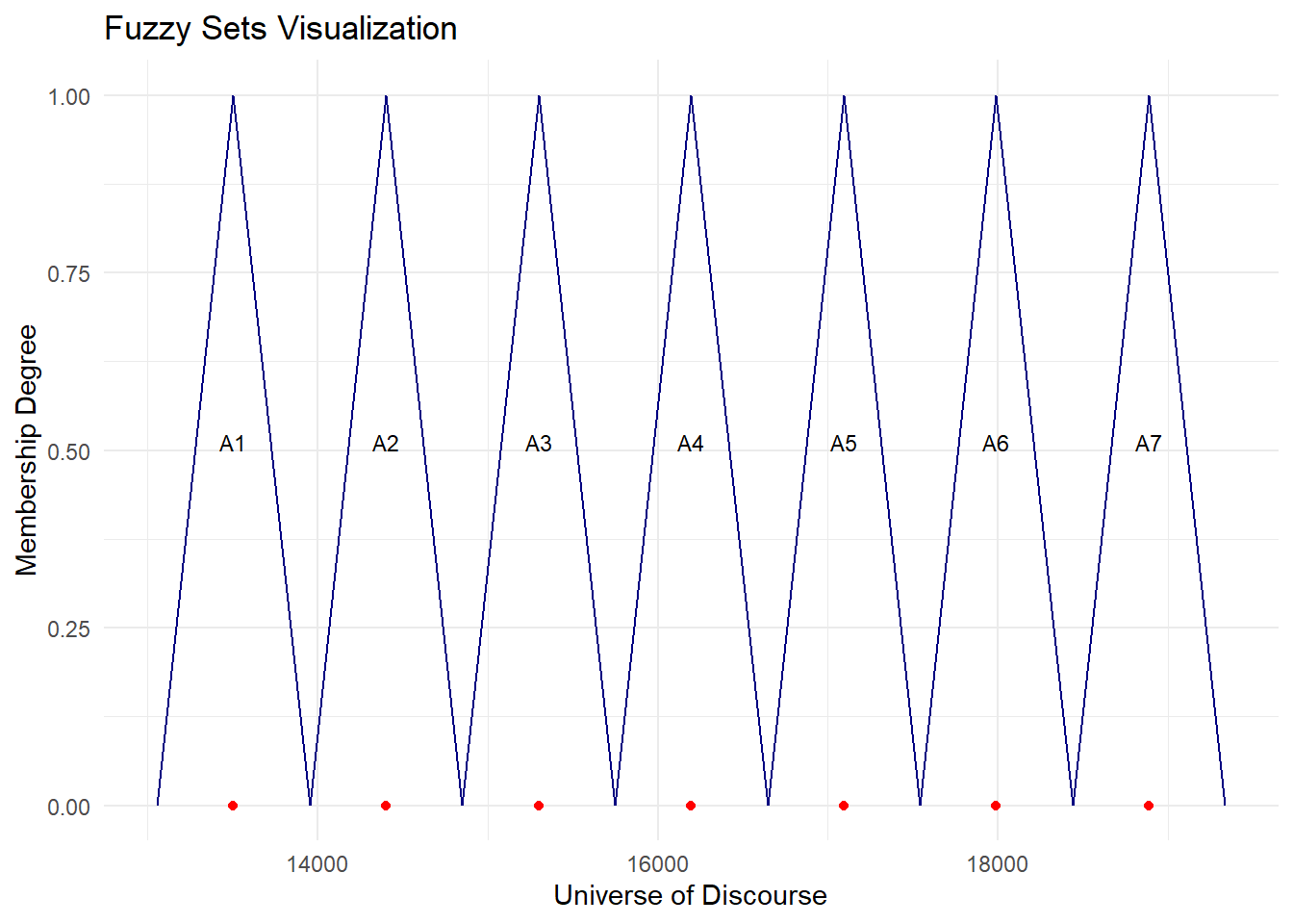

  

Abbasov-Mamedova (2003)

Using fuzzy.ts2() function we can fit the Abbasov-Mamedova model which was developed for demographic forecasting, focusing on handling the uncertainty in population growth.

Step 1 - Define Universe of Discourse (U)

In the research paper, the authors worked on variation in population data, where variation is the first-order differences. In this article, we use the enrollment time series and evaluate the variation in it.

cat('Min diff =',min(diff(enrollment, differences = 1)), 'and Max diff =',
max(diff(enrollment, differences = 1)))

Min diff = -955 and Max diff = 1291

Step 2 - Data partitioning into seven equal intervals

Step 3 - Fuzzification

To determine the membership values we use this formula: \(\mu_{A_i} = \frac{1}{1+[C(U-u_{m^i})]^2}\), where \(u_{m^i}\) is the mid-point of the respective interval. The parameter ‘C’ is a constant which needs to be optimized. So here every year has it’s own fuzzy set representation.

Step 4 - Formulation of Fuzzy Logic Relationship (FLR)

First, we select value of the Basic Parameter ‘w’ which defines how many years of past data should be considered for defining the fuzzy logic relationship. If w = 5, we use 6 past years’ data ( for 5 past differences we require 6 past year data).

• FLR matrix = intersection(Operation matrix, Criteria matrix)

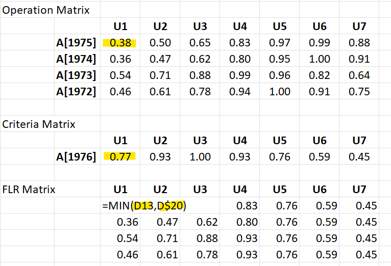
The Operation Matrix contains the fuzzy sets for years t-5, t-4, t-3, t-2 (in each row). The Criteria Matrix is the fuzzy set for year t-1.

Let’s consider year 1997 and w = 5. We can extract the below figures from the model output in R (table 3). The Operation matrix consists of fuzzy sets for years 1992, 1993, 1994, 1995 and Criteria Matrix for year 1996. The FLR Matrix is the result of minimum composition, where we take row-wise minimum over all years.

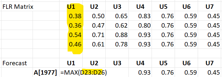
To forecast we take column-wise maximum for each interval. This gives us the fuzzy output set.

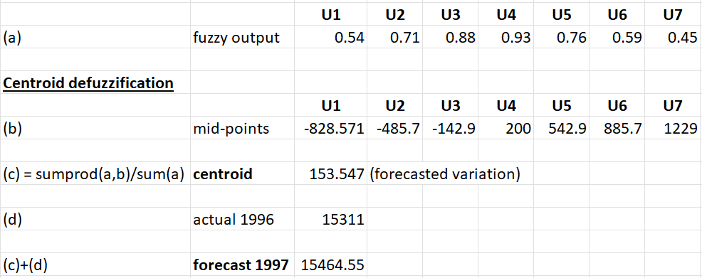
Lastly we need to defuzzify for which we use centroid defuzzification. This gives us the forecasted variation which we can add back to last known actual value of 1996 to get forecasted value of 1997.

In this model we have two parameters ‘w’ (if w = 5, we utilise last 6 years of data) and ‘c’ is a constant which helps determine the shape of the membership values for respective fuzzy sets. The GDOC() commands helps us find the optimal value of parameter ‘c’ by considering n*w number of models. We use MAPE as a criteria to compare these models.

# lets take U = [-1000, 1400]
d1 = 45
d2 = 109

# finding best 'c' value 
# GDOC(enrollment, n = n, w = 5, D1 = d1,D2 = d2, error = 1e-06, CEF = 'MAPE',type = 'Abbasov-Mamedova')  

# Abbasov-Mamedova, 2010 
fit = fuzzy.ts2(enrollment,n = n,w = 5,D1 = d1,D2 = d2,C = 0.000807,        
                forecast = 1,plot = TRUE,trace = T, grid = T,           
                type = "Abbasov-Mamedova")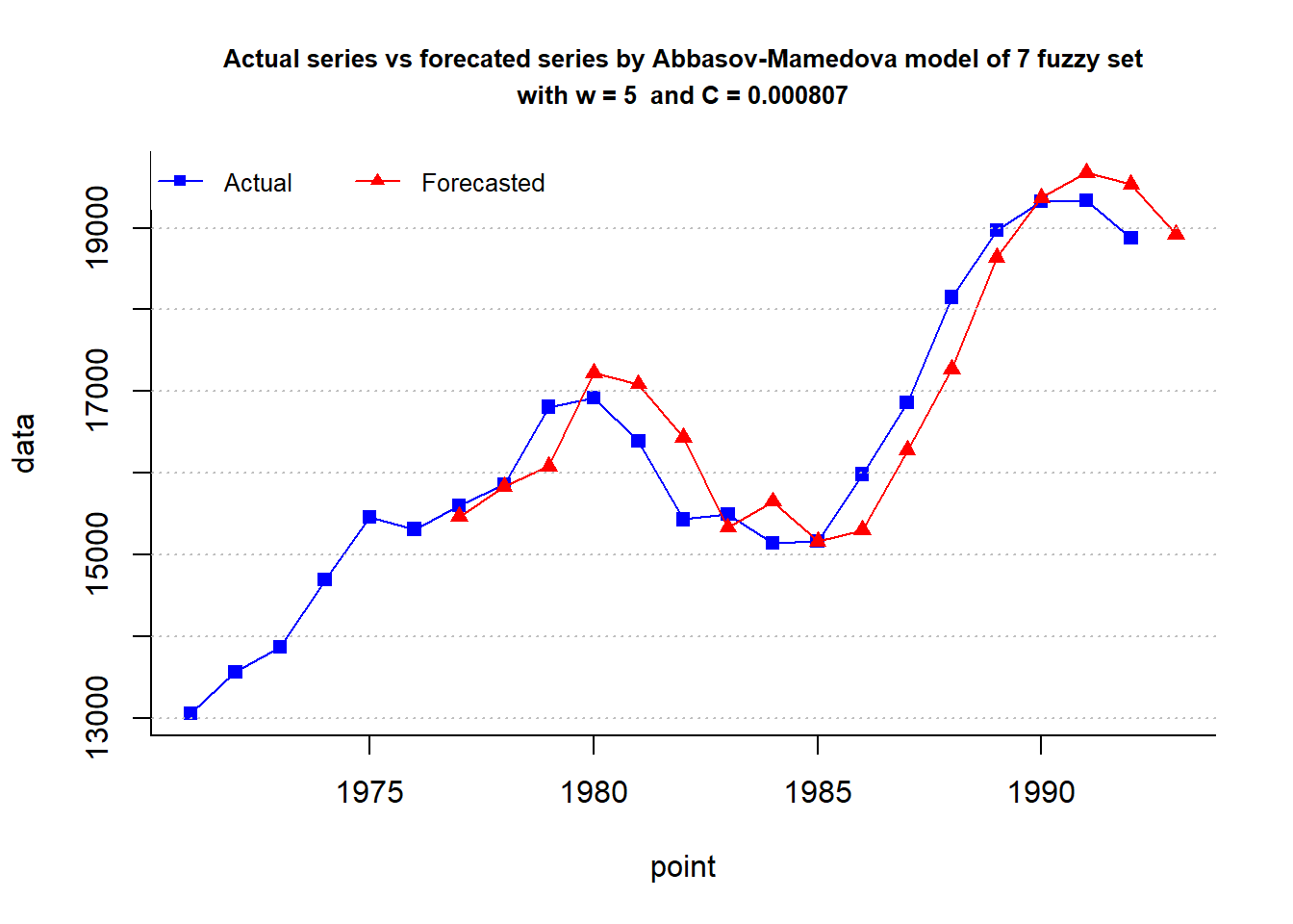 

cat("MAPE =",fit$accuracy[4],"%")

MAPE = 2.63 %

options(digits = 3)
head(fit$table3, 3) # display first 3 years' fuzzy sets

[1] NA                                                                                                                                                     
[2] "A[1972]={(0.462234021634/u1),(0.608610277125/u2),(0.783773469868/u3),(0.941814613024/u4),(0.999209344804/u5),(0.914986378023/u6),(0.747303963181/u7)}"
[3] "A[1973]={(0.544849611404/u1),(0.711161398549/u2),(0.884922664773/u3),(0.993005360421/u4),(0.964175540589/u5),(0.819418828215/u6),(0.642380942176/u7)}"

plot.my.fuzzy.sets(fit$table1)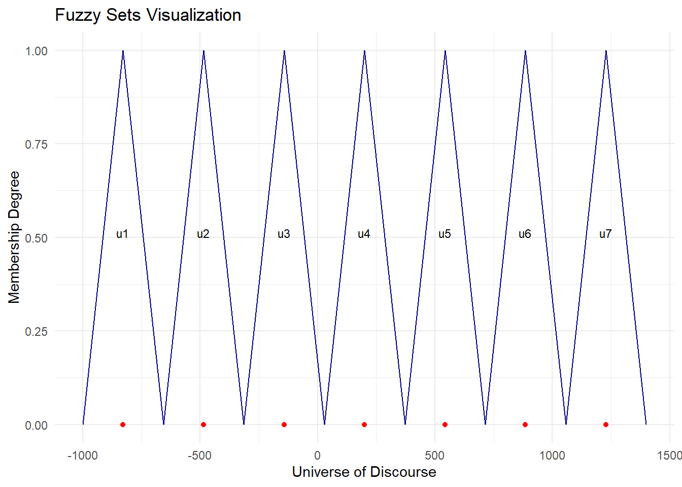

Final Results

Model	MAPE
ARIMA(1,1,0)	2.52 %
Chen	3.11 %
Heuristic	2.45 %
Singh	1.53 %
Chen-Hsu	1.89 %
Abbasov-Mamedova	2.68 %

Exploring Alternatives

Universe of Discourse Alternatives

1st Differences

Let’s explore two alternative ways of defining our Universe of Discourse: (1) Universe is 1st-order differences and, (2) Universe is Percentage-Change. Let’s build Singh Model for both approaches.

# 1st order differences
df = diff(enrollment, differences = 1)
cat("Range of values:",min(df),'to',max(df))

Range of values: -955 to 1291

d1 = 45
d2 = 109
n = 6

fit = fuzzy.ts1(ts = df,n = n,D1 = d1,D2 = d2,                 
                type="Singh",plot=F, trace = T, grid = T) 

pred.og = cumsum(c(enrollment[4], fit$table2['forecasted'][-c(1:3),] ) )[-1]

plot(enrollment, type='l',lwd=2,col='navy',
     xlab='Years',ylab='Enrollments',main='1st order differences')
points(enrollment, cex=0.7,col='navy')
lines(1975:1992, pred.og, col='red', lwd=2)
legend('topleft',c('Actual','Forecast'),col=c('navy','red'),lwd=2,bty='n')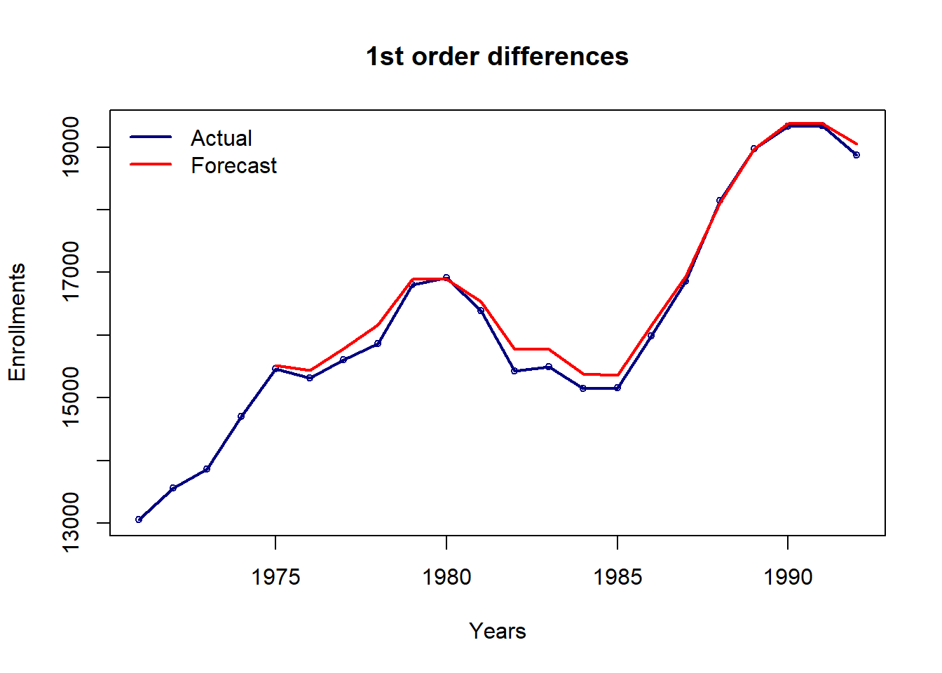

cat("MAPE =",round(100*mape(enrollment[-c(1:4)], pred.og),2),"%")

MAPE = 0.88 %

plot.my.fuzzy.sets(fit$table1)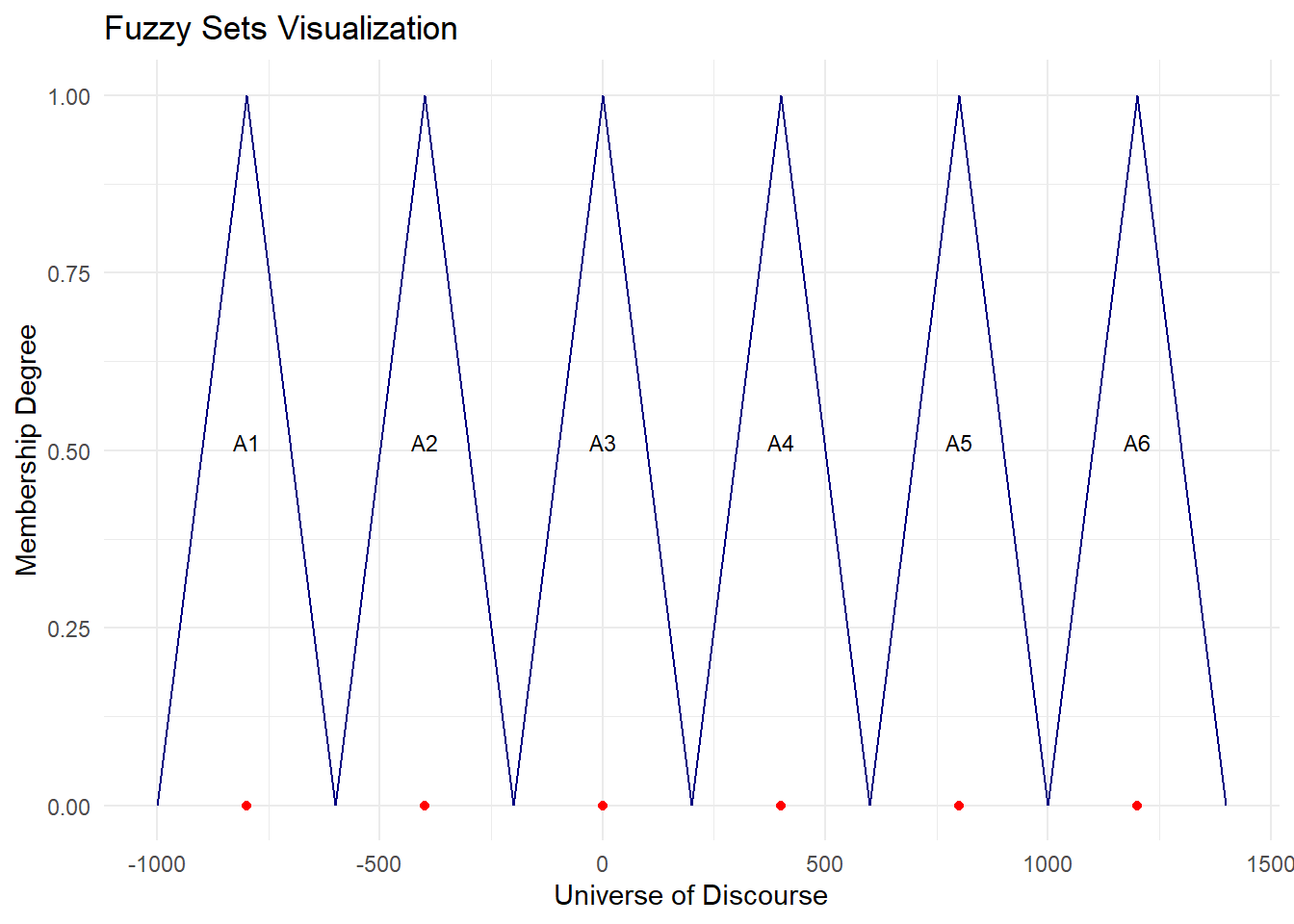

% Differences

# percentage differences
df = diff(enrollment) / lag(enrollment, -1) * 100
cat("Range of values:",min(df),'to',max(df))

Range of values: -5.83 to 7.66

d1 = 0.17
d2 = 0.34
n = 6

fit = fuzzy.ts1(ts = df,n = n,D1 = d1,D2 = d2,                 
                type="Singh",plot=F, trace = T, grid = T) 

pred.changes = na.omit(fit$table2['forecasted'])

preds = numeric(nrow(pred.changes))
preds[1] = enrollment[4]*(1+pred.changes[1,]/100)
for(i in 2:length(preds)){
  preds[i] = preds[i-1]*(1+pred.changes[i,]/100)
}


plot(enrollment, type='l',lwd=2,col='navy',
     xlab='Years',ylab='Enrollments',main='Percentage differences')
points(enrollment, cex=0.7,col='navy')
lines(1975:1992, preds, col='red', lwd=2)
legend('topleft',c('Actual','Forecast'),col=c('navy','red'),lwd=2,bty='n')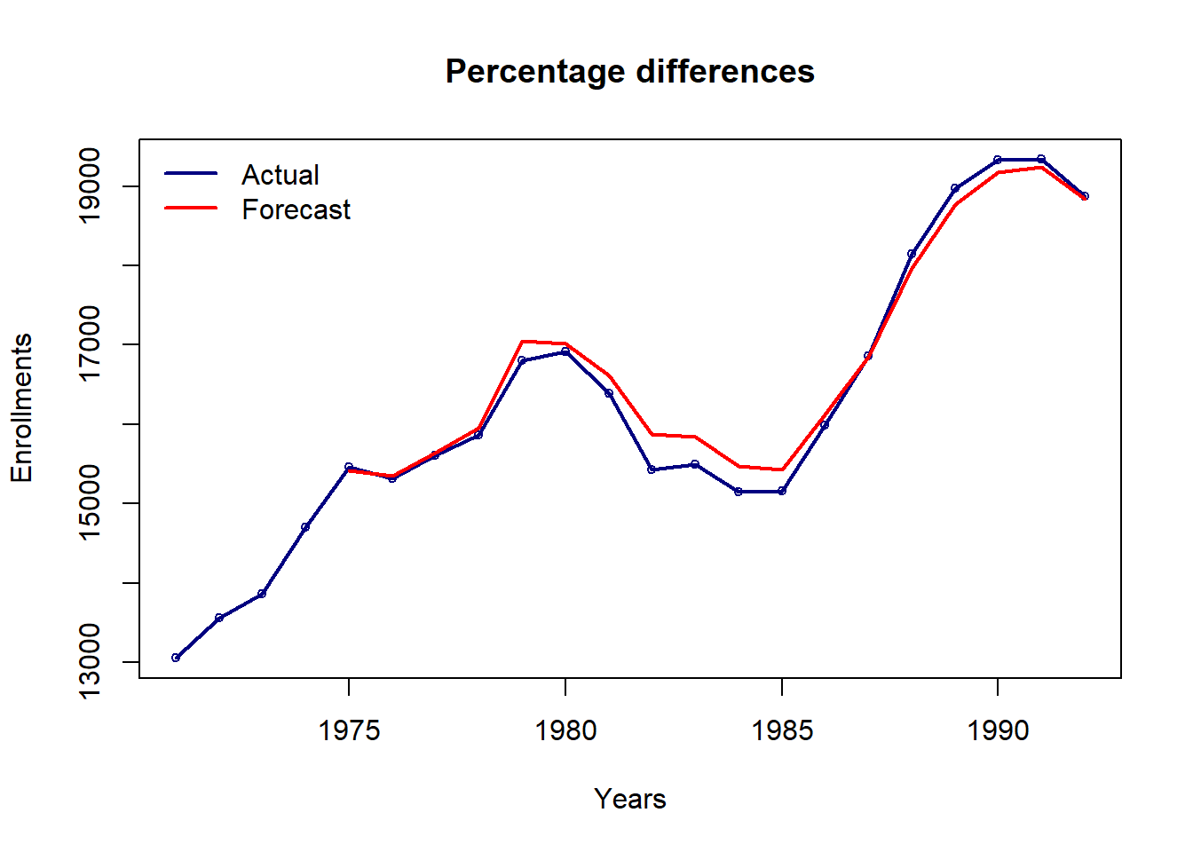

cat("MAPE =",round(100*mape(enrollment[-c(1:4)], preds),2),"%")

MAPE = 1.01 %

plot.my.fuzzy.sets(fit$table1)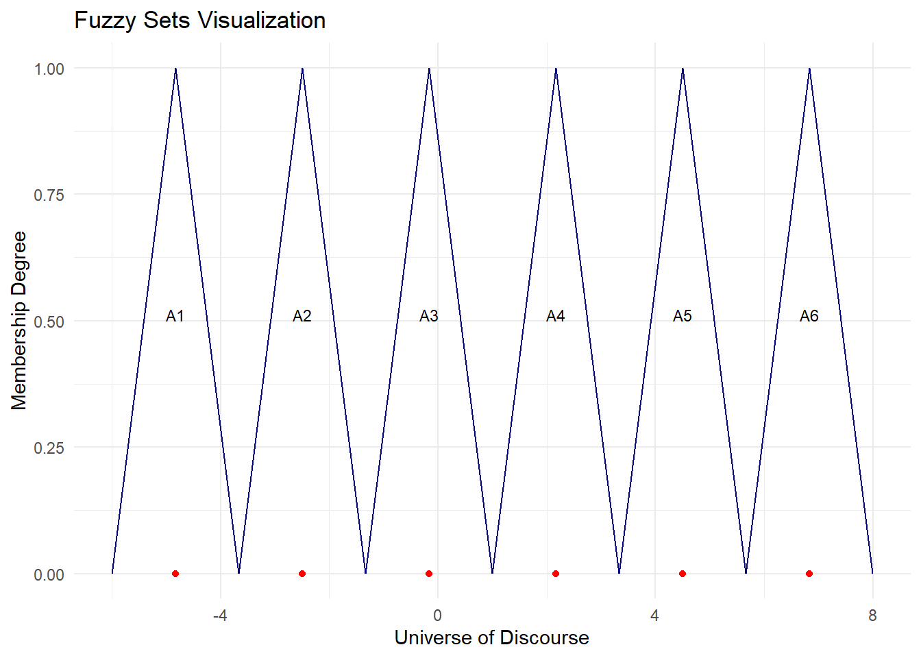

Data Partitioning Alternatives

Let’s explore data partitioning alternatives: (1) Distribution-based (2) Density-based (3) Re-partitioning Discretization and (4) Power of ‘p’ rule.

Distribution-based

# step 1 - evaluate the average of absolute 1st order differences and then half it
df = diff(enrollment, differences = 1)
x = 0.5*mean(abs(df))

# step 2 - evaluate the base
base = function(x){
  ifelse(x>=0.1 & x<=1,0.1,
         ifelse(x>=1.1 & x<=10,1,
                ifelse(x>=11 & x<=100,10,
                       ifelse(x>=101 & x<=1000,100,NA))))
}

# step 3 - interval length, round off using the base
length = round(x/base(x))*base(x)

# step 4 - number of intervals
n = round(7000/length)

# step 5 - FTS Modelling
D1 = 55    
D2 = 663 
fit = fuzzy.ts1(ts = enrollment,n = n,D1 = D1,D2 = D2,                 
                type="Singh",plot=TRUE, trace = T, grid = T)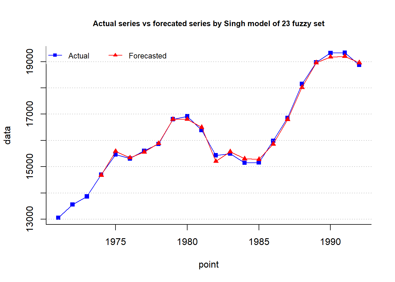 

cat("MAPE =",fit$accuracy[4],"%")

MAPE = 0.558 %

plot.my.fuzzy.sets(fit$table1)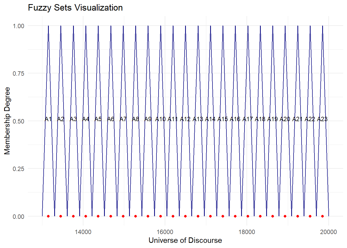

Density-based

# step 1 - partition into equal intervals
D1 = 55    
D2 = 663 
n = 7    # number of intervals/ fuzzy sets  

breaks = seq(13000, 20000, length.out = 8)

df = as.data.frame(table(cut(enrollment, breaks, include.lowest = T)))
df = df[order(-df$Freq),]

as.numeric(head(rownames(df),3)) # intervals 3, 4, 1 -> split 4, 3, 2 times

[1] 3 4 1

# Chen-Hsu, 2004 
A = fuzzy.ts1(enrollment,n = 7,type = "Chen-Hsu",plot = 1) 

B = ChenHsu.bin(A$table1, n.subset = c(2,1,1,4,3,1,1)) 

fit.chen.hsu = fuzzy.ts1(enrollment, type = 'Chen-Hsu', 
                         bin = B, plot = 1, trace = 1)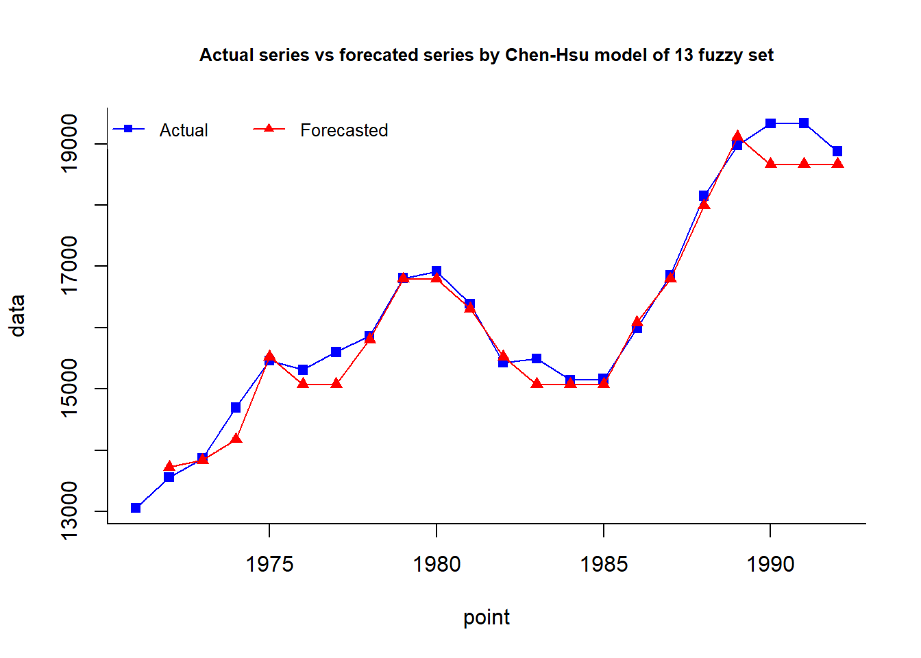 

cat("MAPE =",fit.chen.hsu$accuracy[4],"%")

MAPE = 1.28 %

plot.my.fuzzy.sets(fit.chen.hsu$table1)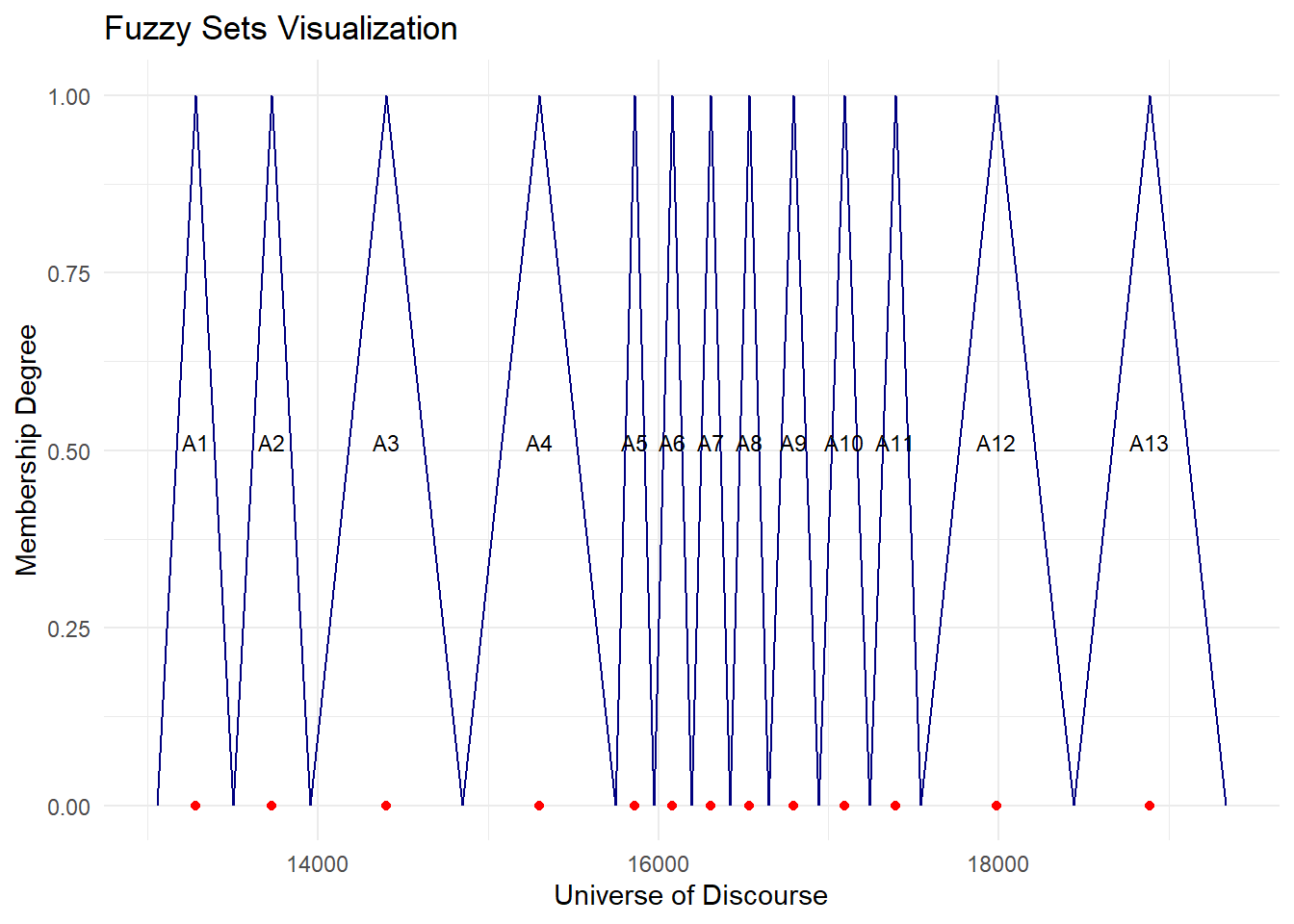

Re-Partitioning Discretization

# number of partitions k = 1 + log_2(sample_size)

D1 = 55    
D2 = 663 
k = round(1 + log(length(enrollment), base = 2))

# Chen, 1996 
fit = fuzzy.ts1(ts = enrollment,n = n,D1 = D1,D2 = D2,
                type = "Singh",plot = TRUE, trace = T, grid = T)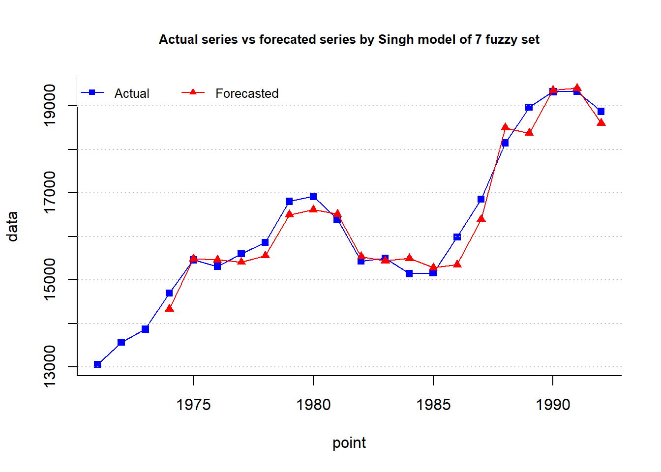 

cat("MAPE =",fit$accuracy[4],"%")

MAPE = 1.53 %

plot.my.fuzzy.sets(fit$table1)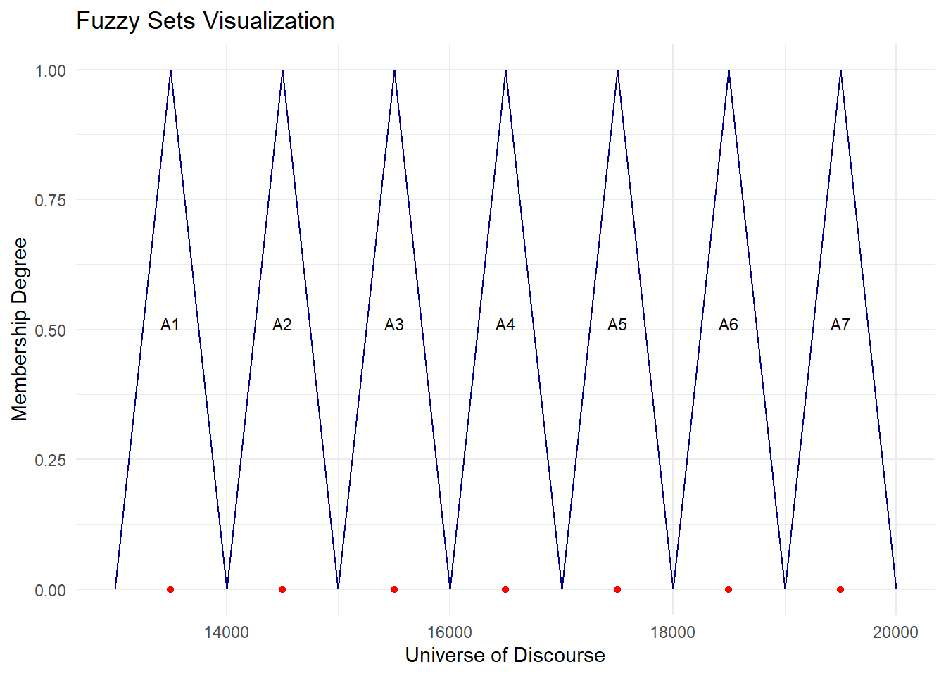

Power of p rule

# Sturges approach or the two power of p rule :
# number of partitions k = 1 + 3.3*log(sample_size)

k = round(1 + log(length(enrollment), base = 2))

cat('Number of intervals :', k)

Number of intervals : 5

Conclusion

This article is part of a comprehensive series on Fuzzy Logic and Systems using R, laying the groundwork for understanding advanced concepts and applications in this field.

For further exploration, you can access other articles in this series:

1. Introduction to Fuzzy Logic in R

2. Fuzzy Logic in R

3. Fuzzy Clustering in R

4. Fuzzy Time Series in R

5. Fuzzy Intelligent Agents

These articles aim to delve deeper into Fuzzy Logic concepts and their practical implementations, building upon the foundation laid by our esteemed professors. Stay tuned for more valuable insights and applications in this exciting field.