Code
import tkinter as tk
import random import math
import numpy as np
import matplotlib.pyplot as plt
import osThis article delves into the sophisticated realm of artificial intelligence by examining how a Fuzzy Logic System (FLS) can enhance the decision-making capabilities of an Intelligent Agent tasked with obstacle navigation. We provide an in-depth analysis of the FLS’s design and its pivotal role in enabling the agent to interpret ambiguous environmental data and make nuanced navigation decisions. The implementation is meticulously crafted in Python, chosen for its efficacy in rapid prototyping and data processing. We demonstrate the agent’s improved performance in a simulated environment, highlighting the FLS’s adaptability and robustness
Intelligent Agents are autonomous AI systems capable of independent action to achieve specific goals. These agents process complex data and employ intricate algorithms to inform their decisions, often interacting within a network that includes humans and other digital systems. This capability enables them to operate effectively in diverse and dynamic environments.
A prominent example is the web crawler, an agent that navigates the internet to index content, employing advanced algorithms to evaluate the relevance and rank of web pages. Similarly, in ‘Smart Grids,’ intelligent agents manage and optimize energy flow, showcasing their significant role in sectors ranging from information technology to energy management. Such applications highlight the broad utility and transformative impact of Intelligent Agents.
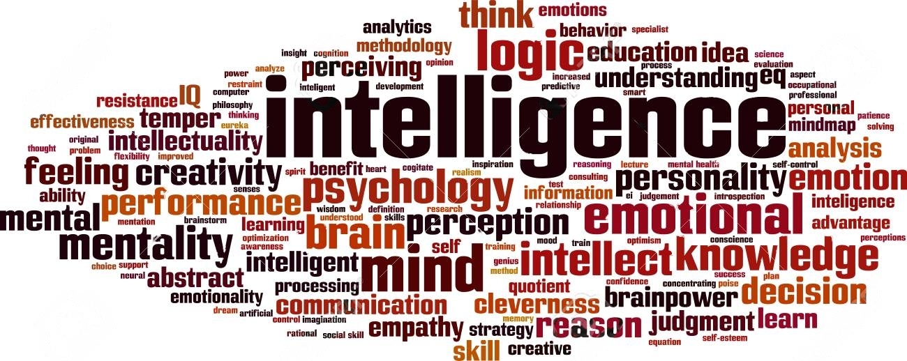
Intelligence is a multifaceted term that invokes a broad spectrum of definitions and associations. Commonly, it brings to mind attributes such as knowledge, understanding, wisdom, logic, and creativity. It encompasses the capacity for reasoning, learning, perception, and problem-solving. Each of these elements contributes to the overarching concept of intelligence, yet they represent only a fraction of its full scope.
To better visualize the expanse of ‘intelligence,’ consider the accompanying word cloud. This visual representation highlights the diversity of terms frequently intertwined with intelligence. It underscores not only cognitive abilities like logic and reasoning but also emotional dimensions such as empathy and self-awareness. The prominence of words like ‘emotional,’ ‘mind,’ ‘psychology,’ and ‘creativity’ within the cloud reflects a modern understanding that intelligence is not solely about intellectual horsepower but also about the harmonious integration of both mental processes and emotional intelligence.
Let’s first form a basic definition of an Intelligent Agent. An intelligent agent is something that takes some information from it’s external environment, does something “intelligent” with it, and then modifies that (or another) environment by it’s actions. This encompasses inputs like sensor readings, language, and emails, and outputs such as motor actions, light signals, or database updates.
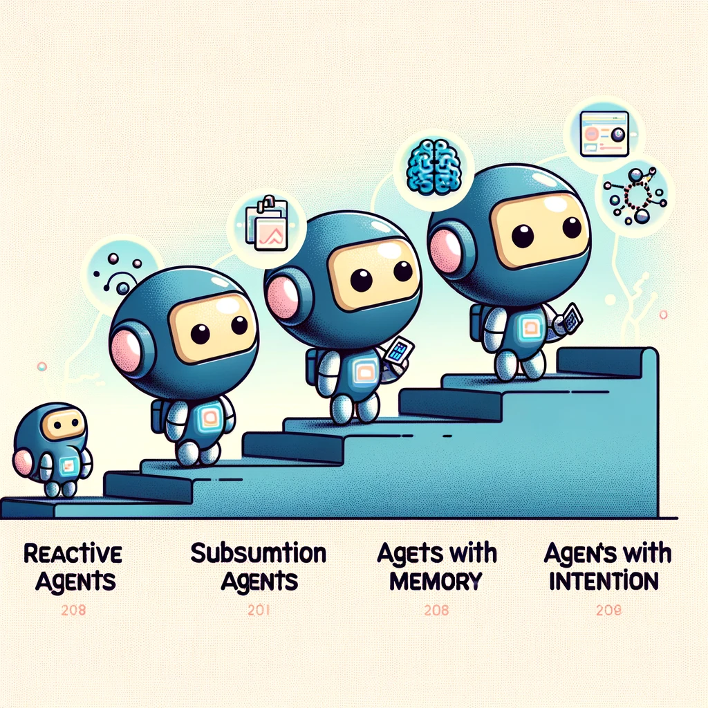
The first kind of Intelligent Agent we come across are called Reactive Agents. These agents are the epitome of simplicity. As the name suggests, they are good are reacting, but to what? They just respond immediately to their environment, making them fast and efficient at dealing with real-time changes. The actions they take are snap-decisions based on current state of their environment.
Let’s consider a simple robot vacuum cleaner. It takes as input, the proximity sensor readings (which tells how far objects are). The intelligence bit here is in choosing a random angle (turning) based on the sensor readings (indicating a nearby obstacle), and the output is turning its motors (to make a turn). When there is no sensor activity, then it follows a background activity, say wandering around the room cleaning dirt.
The next variety is called Sub-Sumption Agents. These agents have a hierarchy of behaviors with different triggers defining how to move from enacting between different behaviors. So, for our vacuum cleaner robot, let’s get it a battery life. When it has sufficient battery (say above 300 units out of 1000), then it continues wandering around the room, but when the battery level falls below 300, its mode of action switches from “random wandering” to “seeking the charger”. This makes our agent adaptive and exhibit goal-oriented behaviors.
So far our agents did not have a concept of time. No past. No future. Only behave and react to present. We might call them mindful agents - ones living in the moment. Now, let’s give them a sense of remembrance. These are Agents with Memory. They remember some inputs, build an idea (say a model, a graph, a structure essentially) about aspects of their external environment, then use it as inputs going forward. They may also remember the relationship between inputs and behaviors/actions taken. This incorporates the ability to remember, plan and solve problems and make more learned/experienced decisions. For example, let’s give our robotic vacuum cleaner a map of the room, so now it has a path to follow rather than randomly wandering about. In it’s reactive form, it must have left some spots dirty.
A more refined approach would be to maintain this ‘memory’ as an external database. Such agents are called Agents with External Memory. The incorporation of memory is the beginning of learning. And the idea of learning becomes more and more important as we develop more sophisticated agents.
Lastly we have Agents with Intention which represent a more advanced tier in the hierarchy of AI systems. They are set with high level descriptions of tasks and using a planning process, with strategies and a preset list of instructions, they work towards a sequence of behaviors. Say now our robotic vacuum cleaner has the ability to recognize the time periods when the house is relatively less crowded, so it adjusts its cleaning schedule accordingly. On encountering a new furniture/obstacle, it not only avoids it but also upgrades the path followed to ensure most efficient cleaning.
A refined approach to creating agents with intention is encapsulated in the Belief, Desire, and Intention (BDI) Model. In this framework, the agent is driven by specific desired outcomes—it harbors desires or goals it seeks to achieve. It possesses beliefs about the world’s current state, including understanding the potential impact of its actions within this environment. Armed with this knowledge, the agent formulates intentions, which are concrete plans of action aimed at bridging the gap between the current reality and its desired goals. This model underscores a sophisticated decision-making process, where the agent continuously assesses its surroundings, aligns its actions with its goals based on its beliefs, and dynamically adapts its strategy to navigate closer to its desired state of the world. We can incorporate Obligations too like ensuring certain safety constraints.
Let’s start by importing some libraries like Tkinter which is used for creating GUI components, random and math for mathematical operations and random number generation, numpy for numerical operations, and matplotlib.pyplot for plotting graphs. Additionally, os is used for operating system dependent functionality, such as file and directory operations.
import tkinter as tk
import random import math
import numpy as np
import matplotlib.pyplot as plt
import osTo simulate the decision-making process of our robot, we introduce a class named Brain. This class acts as the central processing unit, interpreting sensor data and determining the robot’s movements. The brain helps illustrate its function in orchestrating complex behaviors based on inputs and internal logic.
In the __init__ method, we initialize variables such as SpeedL and SpeedR, which are crucial for controlling the robot’s left and right motor speeds, respectively. This setup is foundational, as precise speed control is vital for maneuvering the robot effectively within its environment.
The ThinkAndAct method is where the robot’s sensory inputs are translated into actions. Inputs include LightL and LightR, representing light intensities detected by the left and right sensors, and (x, y), the robot’s current coordinates. These inputs guide the robot in navigating towards or away from light sources and avoiding obstacles by adjusting its trajectory.
class Brain():
    def __init__(self,botp):
        self.bot = botp
        self.speedL = 5
        self.speedR = 5

    # modify this to change the robot's behaviour
    def thinkAndAct(self, lightL, lightR, x, y, sl, sr):
        newX = None
        newY = None

        speedLeft = 10
        speedRight = 10

        # Toroidal geometry
        #------------------------------
        window_width = 1000
        window_height = 750
        newX = x # current x-coordinate
        newY = y # current y-coordinate
        if newX < 0:
            newX = window_width
        elif newX > window_width:
            newX = 0
        if newY < 0:
            newY = window_height
        elif newY > window_height:
            newY = 0

        return speedLeft, speedRight, newX, newY
We now turn our attention to defining the robot itself through a class named Bot. This class encapsulates the essential attributes and behaviors that bring our robot to life in a simulated environment.
The __init__ method sets the foundational parameters of our robot, including its position (x, y), and orientation theta. These initial values are critical for establishing the robot’s starting point and direction in the simulated world.
In the ThinkAndAct method, we leverage the Brain class’s logic to update the robot’s speed and position. This integration embodies the interaction between the robot’s “mind” (the Brain) and its physical “body” (the Bot), allowing for dynamic responses to the environment.
The SenseLight method essentially calculate the distance of the bot from the lamp and then coverts it into intensity, giving us values for LightL & LightR. Then we have the Draw and Move methods which details the bot’s geometric shape, and orientation and handles different movement dynamics respectively.
The Bot class, with its methods, forms the cornerstone of our robot’s functionality in the simulation, blending sensory inputs, decision-making, and physical actions.
class Bot():
    def __init__(self,namep):
        self.name = namep
        self.x = random.randint(100,900)
        self.y = random.randint(100,900)
        self.theta = random.uniform(0.0,2.0*math.pi)
        self.ll = 60 # axle width
        self.sl = 0.0
        self.sr = 0.0

    def thinkAndAct(self, agents, passiveObjects):
        lightL, lightR = self.senseLight(passiveObjects)
        self.sl, self.sr, xx, yy = self.brain.thinkAndAct(lightL, lightR,
                                          self.x, self.y, self.sl, self.sr)
        if xx != None:
            self.x = xx
        if yy != None:
            self.y = yy

    def setBrain(self,brainp):
        self.brain = brainp

    # returns the output from polling the light sensors
    def senseLight(self, passiveObjects):
        lightL = 0.0
        lightR = 0.0
        for pp in passiveObjects:
            if isinstance(pp,Lamp):
                lx,ly = pp.getLocation()
                distanceL = math.sqrt( (lx-self.sensorPositions[0])*(lx-
                self.sensorPositions[0]) + (ly-self.sensorPositions[1])*(ly-
                self.sensorPositions[1]) )

                distanceR = math.sqrt( (lx-self.sensorPositions[2])*(lx-
                self.sensorPositions[2]) + (ly-self.sensorPositions[3])*(ly-
                self.sensorPositions[3]) )

                lightL += 200000/(distanceL*distanceL)
                lightR += 200000/(distanceR*distanceR)
        return lightL, lightR

    def update(self,canvas,dt):
        self.move(canvas,dt)

    ## draw method ...

    ## move method ...
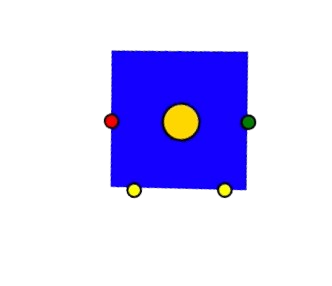
The draw method visualizes the robot on the canvas, calculating its geometric shape based on its position (x, y) and orientation (theta). It creates a polygon representing the robot’s body and ovals for its central position, wheels, and sensors, using trigonometric functions to determine their exact locations. The colors differentiate parts: the body is blue, the center is gold, wheels are red and green, and sensors are yellow. This method is crucial for visually tracking the robot’s movement and orientation within the simulation environment.
# draws the robot at its current position
def draw(self,canvas):
  # calculate vertices of robot's polygon shaped body
    points = [
    (self.x + 30*math.sin(self.theta)) - 30*math.sin((math.pi/2.0)-self.theta),
    (self.y - 30*math.cos(self.theta)) - 30*math.cos((math.pi/2.0)-self.theta),
    (self.x - 30*math.sin(self.theta)) - 30*math.sin((math.pi/2.0)-self.theta),
    (self.y + 30*math.cos(self.theta)) - 30*math.cos((math.pi/2.0)-self.theta),
    (self.x - 30*math.sin(self.theta)) + 30*math.sin((math.pi/2.0)-self.theta),
    (self.y + 30*math.cos(self.theta)) + 30*math.cos((math.pi/2.0)-self.theta),
    (self.x + 30*math.sin(self.theta)) + 30*math.sin((math.pi/2.0)-self.theta),
    (self.y - 30*math.cos(self.theta)) + 30*math.cos((math.pi/2.0)-self.theta)
    ]
    canvas.create_polygon(points, fill="blue", tags=self.name)
  # calculate robot's sensor's positions relative to it's body
    self.sensorPositions = [
    (self.x + 20*math.sin(self.theta)) + 30*math.sin((math.pi/2.0)-self.theta),
    (self.y - 20*math.cos(self.theta)) + 30*math.cos((math.pi/2.0)-self.theta),
    (self.x - 20*math.sin(self.theta)) + 30*math.sin((math.pi/2.0)-self.theta),
    (self.y + 20*math.cos(self.theta)) + 30*math.cos((math.pi/2.0)-self.theta)
    ]

    centre1PosX = self.x
    centre1PosY = self.y
    # circle representing the center - gold color
    canvas.create_oval(centre1PosX-8,centre1PosY-8,
                       centre1PosX+8,centre1PosY+8,fill="gold",tags=self.name)
    # circle representing the wheels - red & green color
    wheel1PosX = self.x - 30*math.sin(self.theta)
    wheel1PosY = self.y + 30*math.cos(self.theta)
    canvas.create_oval(wheel1PosX-3,wheel1PosY-3,wheel1PosX+3,
                       wheel1PosY+3,fill="red",tags=self.name)

    wheel2PosX = self.x + 30*math.sin(self.theta)
    wheel2PosY = self.y - 30*math.cos(self.theta)
    canvas.create_oval(wheel2PosX-3,wheel2PosY-3,wheel2PosX+3,
                       wheel2PosY+3,fill="green",tags=self.name)
    # circle representing the sensors - yellow color
    sensor1PosX = self.sensorPositions[0]
    sensor1PosY = self.sensorPositions[1]
    sensor2PosX = self.sensorPositions[2]
    sensor2PosY = self.sensorPositions[3]
    canvas.create_oval(sensor1PosX-3,sensor1PosY-3,
      sensor1PosX+3,sensor1PosY+3, fill="yellow",tags=self.name)
    canvas.create_oval(sensor2PosX-3,sensor2PosY-3,
      sensor2PosX+3,sensor2PosY+3, fill="yellow",tags=self.name)
The move function updates the robot’s position and orientation based on its left and right speeds (sland sr). It calculates the radius of the curve (R) the robot is moving along and the angular velocity (omega). The robot’s new position (newX, newY) and orientation (newTheta) are determined by applying a rotation matrix to account for the movement over a small time step (dt). This method ensures the robot moves realistically, simulating turning and straight-line movement based on differential wheel speeds.
def move(self,canvas,dt):
    if self.sl==self.sr:
        R = 0
    else:
        R = (self.ll/2.0)*((self.sr+self.sl)/(self.sl-self.sr))
    omega = (self.sl-self.sr)/self.ll
    ICCx = self.x-R*math.sin(self.theta) #instantaneous centre of curvature
    ICCy = self.y+R*math.cos(self.theta)
    m = np.matrix( [ [math.cos(omega*dt), -math.sin(omega*dt), 0],
        [math.sin(omega*dt), math.cos(omega*dt), 0],  [0,0,1] ] )
    v1 = np.matrix([[self.x-ICCx],[self.y-ICCy],[self.theta]])
    v2 = np.matrix([[ICCx],[ICCy],[omega*dt]])
    newv = np.add(np.dot(m,v1),v2)
    newX = newv.item(0)
    newY = newv.item(1)
    newTheta = newv.item(2)
    newTheta = newTheta%(2.0*math.pi)
    # ^ make sure angle doesn't go outside [0.0,2*pi)
    self.x = newX
    self.y = newY
    self.theta = newTheta
    if self.sl==self.sr: # straight line movement
        self.x += self.sr*math.cos(self.theta) #sr wlog
        self.y += self.sr*math.sin(self.theta)
    canvas.delete(self.name)
    self.draw(canvas)
Let’s now define some obstacles, by defining a class called Lamp. Here we initialise the coordinates such that the lamps are placed randomly across the window. Using the Draw method we define a red oval shape with an ‘x’ in the center.
class Lamp():
    # define initial position of lamps
    def __init__(self,namep):
        self.centreX = random.randint(100,900)
        self.centreY = random.randint(100,650)
        self.name = namep

    def draw(self,canvas):
        radius = 10
        body = canvas.create_oval(self.centreX-10,self.centreY-10,
                                  self.centreX+10,self.centreY+10,
                                  fill="red",tags=self.name)
        body = canvas.create_text(self.centreX, self.centreY,
            text='X',anchor='center',font=('Arial',int(radius)), tags=self.name)

    def getLocation(self):
        return self.centreX, self.centreY
In addition to the classes that model our robot’s brain and body, we need to establish some foundational functions that support the robot’s interaction with its environment.
The first function we introduce is responsible for initialising the graphical window where our robot will navigate and interact. This setup is crucial for visualizing the robot’s movements and the environment it explores.
To interact with the simulation and directly influence the robot’s position, we implement a buttonClicked function. This function dictates the robot’s response to mouse clicks within the environment, allowing us to relocate the robot on demand. Currently, when a user clicks somewhere within the environment, this function repositions the robot to the specified coordinates.
def initialise(window):
    window.resizable(False,False)
    canvas = tk.Canvas(window,width=1000,height=750)
    canvas.pack()
    return canvas

def buttonClicked(x,y,agents):
    for rr in agents:
        if isinstance(rr,Bot):
            rr.x = x
            rr.y = y
The next function createObjects initializes the simulation environment by creating specified numbers of robotic agents (Bot instances) and passive objects (Lamp instances), then visually represents them on a canvas. Each robot is given a unique name and associated with a Brain object to process inputs and control movement. Similarly, each lamp is named and placed in the environment. The function also prepares for user interaction by enabling a click event on the canvas, allowing dynamic interaction during the simulation.
def createObjects(canvas,noOfBots,noOfLights):
    agents = [] # list of bot instances
    passiveObjects = [] # list of Lamp instances
    for i in range(0,noOfBots):
        bot = Bot("Bot"+str(i))
        brain = Brain(bot)
        bot.setBrain(brain)
        agents.append(bot)
        bot.draw(canvas)
    for i in range(0,noOfLights):
        lamp = Lamp("Lamp"+str(i))
        passiveObjects.append(lamp)
        lamp.draw(canvas)
    canvas.bind( "<Button-1>", lambda event: buttonClicked(event.x,event.y,agents))
    return agents, passiveObjects
The moveIt function iterates over each robotic agent (agents), invoking their decision-making and movement processes based on the current environment (passiveObjects). Each agent assesses its situation, decides on a course of action, and updates its position on the canvas. The function recursively schedules itself to run every 25 milliseconds, creating a continuous simulation loop.
The main function sets up the simulation environment. It initializes the main window and canvas, creates the specified number of agents and lights within the environment, and starts the simulation by calling moveIt. This initiates the agents’ interactions within the simulation, continuously updating their states and the visual representation on the canvas. The window.mainloop() call keeps the application running, allowing for dynamic interactions and updates within the simulation.
def moveIt(canvas,agents,passiveObjects):
    for rr in agents:
        rr.thinkAndAct(agents,passiveObjects)
        rr.update(canvas,1.0) # 1.0 is time step dt
    canvas.after(25,moveIt,canvas,agents,passiveObjects)

def main():
    window = tk.Tk()
    canvas = initialise(window)
    agents, passiveObjects = createObjects(canvas,noOfBots=1,noOfLights=8)
    moveIt(canvas,agents,passiveObjects)
    window.mainloop() # allows the window to run unlimited by performing above 2 steps in loop

main()Let’s construct our Fuzzy Logic System tailored to avoid obstacles in the path of our robot. We consider as inputs, the sensor readings from the Left and Right sensors which detect how far the obstacles are. These readings are categorized into three fuzzy sets: {“near”, “too near”, “far”} capturing the proximity to an obstacle.
The Input Domain ranges for our sensors is defined from 0 to 250 units, with these values inversely proportional to the square of distance from the obstacles - representing a range from a close 28 pixels to effectively an Infinite distance.
The system’s output, which dictates the necessary speed adjustments, falls within a domain ranging from -15 to 15 units of speed change, represented by three fuzzy sets: {“decrease”,“no change”,“increase”}.
Our fuzzy rules are set as follows:
The bot then adjusts its trajectory by adding or subtracting the defuzzified speed change values to the left and right motors’ speeds, respectively, ensuring smooth navigation around obstacles.
input_domain = np.arange(0, 250, 0.01)
output_domain = np.arange(-15, 15, 0.01)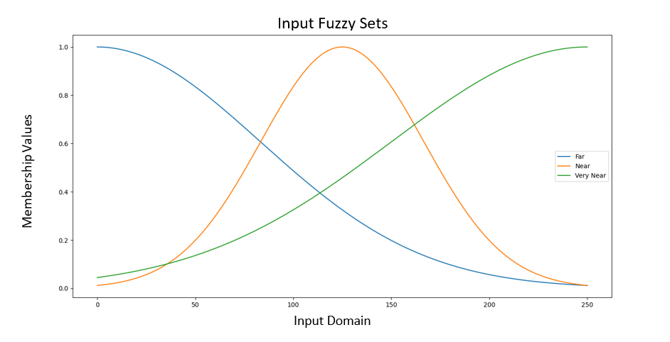
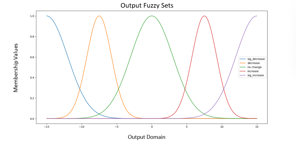
These graphs will help in visualizing how your FLS translates sensor readings into motion decisions, by mapping real-world sensor values to fuzzy linguistic terms, and then to actionable speed changes through the process of fuzzification, rule evaluation, and defuzzification.
First we create a class called FuzzyLogicController with __init__ method where we initialise the input and output domain. Then we have our input and output membership functions followed by another function called fuzzyInf . Here, we take light sensor inputs and evaluate the firing strengths and final output fuzzy set. Lastly, we have our defuzzify function which evaluates the centroid.
class FuzzyLogicController:
    def __init__(self, input_domain, output_domain):
        self.input_domain = input_domain
        self.output_domain = output_domain

    def gaussian_mf(self, x, mean, sigma):
        return np.exp(-np.power(x-mean,2.)/(2*np.power(sigma, 2.)))

    def very_near(self, x):
        return self.gaussian_mf(x, mean = 250, sigma = 100)
    def near(self, x):
        return self.gaussian_mf(x, mean = 125, sigma = 250/6)
    def far(self, x):
        return self.gaussian_mf(x, mean = 0, sigma = 250/3)
        # return np.where(x>5, self.gaussian_mf(x, mean = 0, sigma = 100), 0)

    def sig_increase(self,x):
        return self.gaussian_mf(output_domain, mean = 15, sigma = 3)
    def increase(self,x):
        return self.gaussian_mf(output_domain, mean = 7.5, sigma = 1.75)
    def no_change(self,x):
        return self.gaussian_mf(output_domain, mean = 0, sigma = 3)
    def decrease(self,x):
        return self.gaussian_mf(output_domain, mean = -7.5, sigma = 1.75)
    def sig_decrease(self,x):
        return self.gaussian_mf(output_domain, mean = -15, sigma = 3)

    def fuzzy_inf(self, LightL, LightR):
        rule1 = min(self.near(LightL),self.far(LightR))
        rule2 = min(self.far(LightL), self.near(LightR))
        rule3 = min(self.far(LightL), self.far(LightR))
        rule4 = self.very_near(LightL)
        rule5 = self.very_near(LightR)

        final_decrease = np.fmin(self.decrease(output_domain), rule2)
        final_increase = np.fmin(self.increase(output_domain), rule1)
        final_no_change = np.fmin(self.no_change(output_domain), rule3)
        final_sig_decrease = np.fmin(self.no_change(output_domain), rule4)
        final_sig_increase = np.fmin(self.no_change(output_domain), rule5)

        final = np.maximum.reduce([final_decrease, final_increase,
                    final_no_change,final_sig_decrease,final_sig_increase])
        fired_rules = f"Firing Strengths of rule 1:{rule1:.2f}, \
                        rule 2:{rule2:.2f}, rule 3:{rule3:.2f}, \
                        rule 4:{rule4:.2f}, rule 5:{rule5:.2f}."
        return final, fired_rules

    def defuzzify(self, x, mf):
        numerator = np.sum(mf * x)
        denominator = np.sum(mf)
        return 0 if denominator == 0 else numerator / denominator
Now all we need is to adapt our Brain class so that it is integrated with the FLS system above and produces a graph showing how the rules are fired and output is produced as the bot is moving.
class Brain():

    def __init__(self,botp):
      # existing code
      self.fuzzy_logic_controller = FuzzyLogicController(input_domain,
                                                            output_domain)
      self.init_plot() # function defined below
      # set output directory to save plots
      self.output_dir = 'C:/Users/KUNAL/Downloads/Spring Sem/ \
                        Designing Intelligent Agents/fuzzy logic/plots'

      if not os.path.exists(self.output_dir): # make folder if does not exist
          os.makedirs(self.output_dir)
      self.plot_counter = 0  # To keep track of the plot number

    def init_plot(self):
        self.fig, self.axs = plt.subplots()
        #plt.ion() # to make the plot interactive
        # ^ Initialize an empty line for fuzzy output
        self.line, = self.axs.plot([], [], 'r-', animated = True,
                                   label='Fuzzy Output')
        # Initial centroid line
        self.centroid_line = self.axs.axvline(x=0, color='b', label='Centroid')

        self.axs.set_title('', fontsize=10)
        self.fig.suptitle('Fuzzy Output & Centroid', fontsize=15)
        self.axs.set_xlabel('Speed Change')
        self.axs.set_ylabel('Membership Degree')
        self.axs.legend()
        plt.show(block=False)

    def save_plot(self):
        plot_filename = f"plot_{self.plot_counter}.png"
        plt.savefig(os.path.join(self.output_dir, plot_filename))
        print(f"Saved {plot_filename}")
        self.plot_counter += 1

    def thinkAndAct(self, lightL, lightR, x, y, sl, sr):
        newX = None
        newY = None

        fuzzy_output, fired_rules = self.fuzzy_logic_controller.fuzzy_inf(lightL,
                                    lightR)
        centroid = self.fuzzy_logic_controller.defuzzify(output_domain,
                                    fuzzy_output)
        # Update the plot with the new fuzzy output and centroid
        self.axs.clear()     # Clear previous plot
        self.line, = self.axs.plot(output_domain, fuzzy_output, 'r-',
                                    label='Fuzzy Output')
        self.centroid_line = self.axs.axvline(x=centroid, color='b',
                                              label=f'Centroid = {centroid:.2f}')
        self.axs.set_title(fired_rules, fontsize=10)
        self.fig.suptitle('Fuzzy Output & Centroid', fontsize=15)
        self.axs.set_xlabel('Speed Change')
        self.axs.set_ylabel('Membership Degree')
        self.axs.legend()
        plt.draw()
        plt.pause(0.0001)  # Short pause to allow the plot to update
        if centroid > 1 or centroid < -1: # save only if -1 < centroid value < 1
            self.save_plot()

        # adjust speed with respect to centroid
        # we multiply with 10 to amplify the centroid value
        speedLeft = 10 + 10*centroid
        speedRight = 10 - 10*centroid

        # remaining code
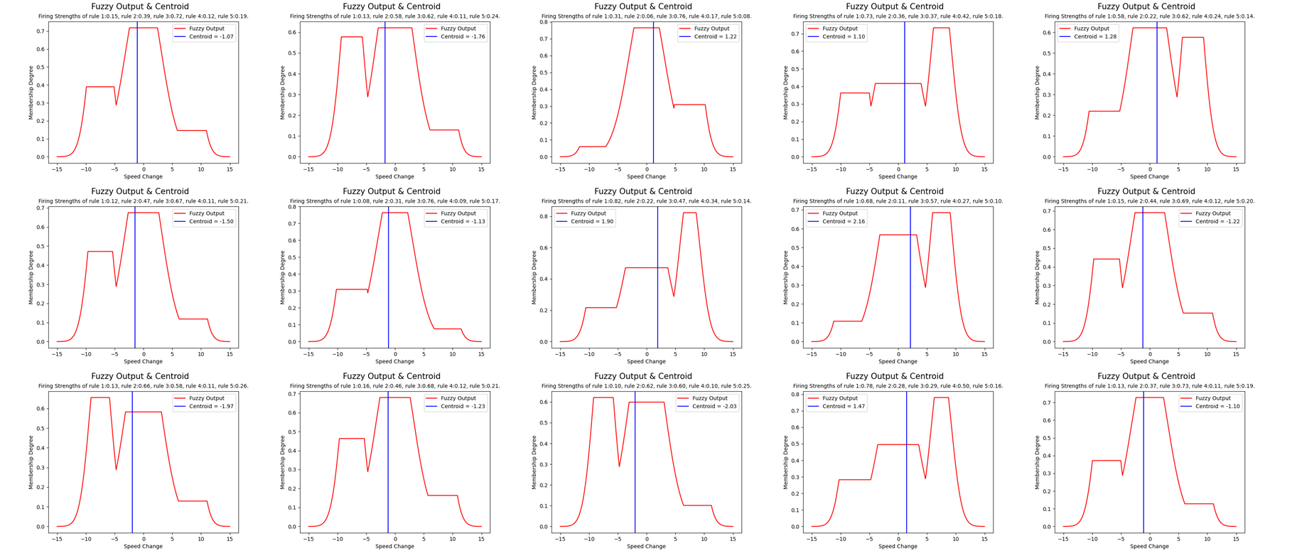
Let’s observe our bot in action. The simulation was conducted four times, each with obstacles randomly placed to test the bot’s adaptability. Accompanying GIFs capture the bot’s maneuvers, offering a dynamic view of its responses in varied scenarios. Additionally, we have visual data representations that plot the fuzzy output set, the resulting centroid values, and the specific rules activated as the bot navigates its environment. This comprehensive analysis will help us understand the effectiveness of our Fuzzy Logic System in real-time decision-making.
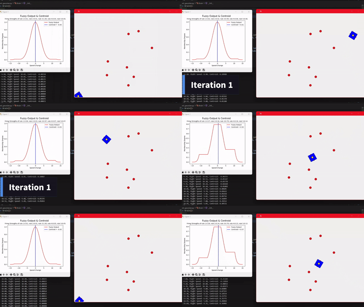
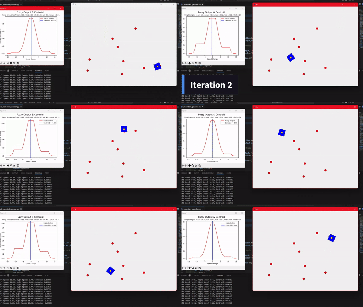
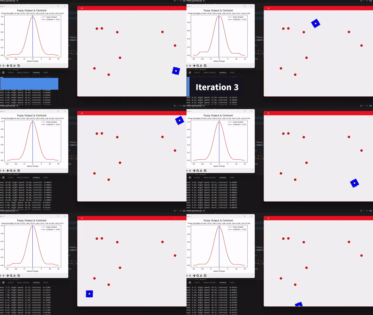
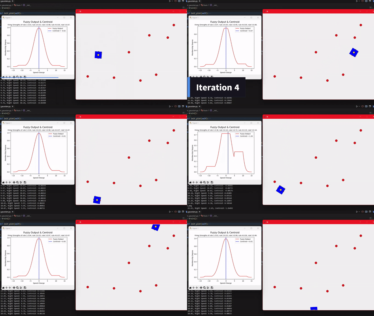
Let’s look at some graphs that we saved…
This article is part of a comprehensive series on Fuzzy Logic and Systems using R, laying the groundwork for understanding advanced concepts and applications in this field.
For further exploration, you can access other articles in this series:
The work in this article is inspired by the teachings of my Professors at the University of Nottingham. Their guidance and expertise have greatly influenced the content and direction of these articles. For further insights into their research and contributions, you can visit their University of Nottingham profiles:
These articles aim to delve deeper into Fuzzy Logic concepts and their practical implementations, building upon the foundation laid by our esteemed professors. Stay tuned for more valuable insights and applications in this exciting field.