This article delves into the realm of fuzzy clustering in R, focusing on two prominent clustering algorithms: k-means and fuzzy c-means. Through practical implementation and analysis, we aim to explore the performance of these algorithms in clustering data sets.
Clustering
In Machine Learning, there is a branch of algorithms dealing with grouping similar data instances to aid in understanding and exploring the underlying patterns in data. Clusters are identified by the algorithms that iteratively try to partition the dataset into subsets based on similarity criterion, with the goal of maximizing intra-cluster similarity and minimizing inter-cluster similarity. Among the most recognized clustering algorithms are K-means, hierarchical clustering, and DBSCAN, each offering unique advantages tailored to specific types of data and application requirements.
Clustering finds its application in a variety of fields, showing its versatility as a tool in the machine learning toolkit. For instance, in market segmentation, clustering helps businesses identify distinct customer groups to tailor marketing strategies effectively. In social network analysis, it can uncover communities or groups based on interaction patterns. Search result grouping utilizes clustering to enhance user experience by organizing similar results, while in medical imaging, it aids in identifying regions of interest or abnormalities. Moreover, clustering plays a crucial role in anomaly detection by isolating outliers that do not fit into any known group, highlighting potential issues or novel findings.
Through these diverse applications, clustering not only enhances our ability to interpret large and complex datasets but also opens avenues for innovation across various sectors, from enhancing consumer engagement strategies to advancing medical research and beyond.
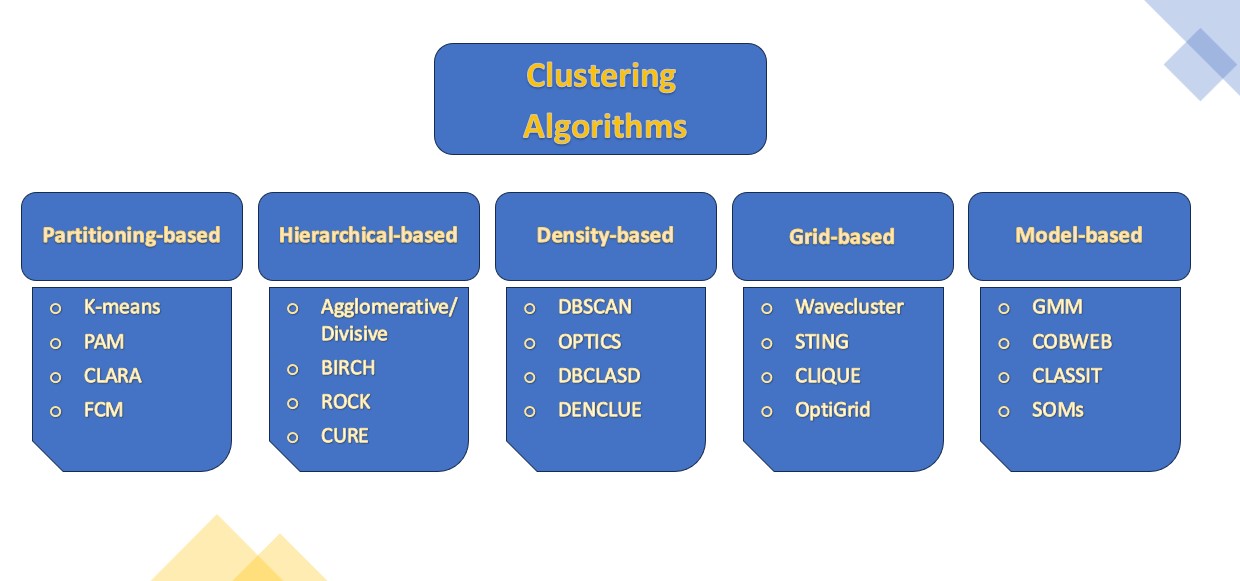
Types of Clustering Models
Partitioning-based models divide the data into clusters based on a similarity or distance metric.
Hierarchical-based models create a hierarchy of clusters that can be represented as a dendrogram. These models are either agglomerative, where each data point is initially considered as a separate cluster and then merged with its closest neighbor, or divisive, where all data points are initially considered as a single cluster, and then the algorithm recursively divides the cluster into smaller sub-clusters.
Density-based models group data points based on their local density. The algorithm identifies regions of high density and separates them from regions of low density.
Grid-based models divide the data space into a finite number of cells representing clusters.
Model-based techniques assume that the data is generated from a mixtures of probability distributions and the goal is to estimate parameters of these distributions.
K-means Clustering
K-means clustering stands as a cornerstone in the realm of unsupervised machine learning, renowned for its simplicity and efficiency. It aims to partition the data into ‘k’ distinct, non-overlapping clusters. The key steps of the K-means algorithm are as follows:
Initialize - we start by randomly selecting ‘k’ initial cluster centers.
Assignment - for each data point, we calculate the distance from each selected center and assign to the closest one.
Update - we re-calculate the centers for each cluster by taking mean of all data points in that cluster.
Repeat steps 2 and 3 until convergence - the algorithm stops iterating once the mean of clusters are no longer changing or maximum iterations are reached.
Quality assessment - we evaluate the inter- and intra-cluster similarity using various metrics.
Fuzzy C-Means
Fuzzy C-Means (FCM) is an extension of traditional clustering algorithms that allows for a more nuanced and flexible definition of cluster membership. Here we allow data points to belong to multiple clusters simultaneously with varying degrees of membership.
This approach is particularly useful in scenarios where the boundaries between clusters are not clearly defined, allowing for a more flexible and often more realistic representation of data groupings. Fuzzy clustering is applied in various fields such as pattern recognition, image processing, and bioinformatics, where it helps to handle the inherent ambiguity and overlap in real-world data.
Below are the steps of Fuzzy C-Means algorithm:
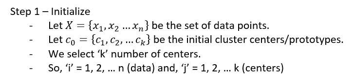
Initialize - we start by randomly selecting ‘c’ initial cluster centers.
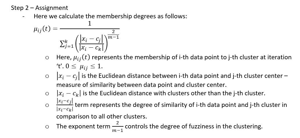
Assignment - for each data point, we calculate the membership value which indicates the degree of belongingness of each point to each cluster.
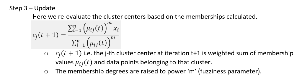
Update - we re-evaluate cluster centers based on membership values. The cluster center is calculated as the weighted mean of all data points where weights are the membership values.
Repeat steps 2 and 3 until convergence - the algorithm stops iterating once the membership values are no longer changing or maximum iterations are reached.
Quality assessment - we evaluate the inter- and intra-cluster similarity using various metrics.
Soft clustering i.e. each data point is belongs to multiple clusters with varying degrees of membership.
This allows for more flexibility in capturing uncertainty and ambiguity in data.
Hard clustering i.e. each data point belongs to only one cluster.
Performs poorly in case of overlapping clusters.
Cluster Shape
Cluster shapes are flexible.
Assumes speherical cluster shapes which may not be appropriate for all datasets.
Outlier sensitivity
Better at dealing with outliers, as can be assigned low membership values to all clusters.
Sensitive to outliers.
Robustness
Less sensitive to noise in the dataset due to soft assignment.
Sensitive to noise in the dataset.
Computation
Computationally intensive due to iterative nature of the algorithm & the need to evaluate membership degrees for each data point.
Less intensive than fuzzy c-means as it involves simpler calculations.
Sensitivity to Initialisation
Less sensitive to initialization due to soft assignment. However, choice of initial membership values and cluster centroids can greatly affect the final results.
More sensitive to initialization.
Interpretability
Provides a more nuanced understanding of our data, revealing degrees of association between data and clusters, which can be where data points naturally belong to more than one group.
Produces a clear-cut, easily interpretable partitioning of the dataset into distinct groups.
Determination of number of clusters
The number of clusters needs to be determined before running the algorithm. This can be a challenge for large data sets where the number of clusters is not known beforehand.
Same
Mall Customers
This dataset (from Kaggle) is aimed to perform Market Basket Analysis to understand the sales behavior of customer over different products and Customer Segmentation to understand the behavior of customers over different aspects. We have Customer ID, Gender, Age, Annual Income and Spending (calculated as Spending score*150).
The aim is to develop a Fuzzy Logic System to analyse and evaluate customer spending behavior in comparison with other machine learning algorithms like Linear Regression, K-means and Random Forest.
Let’s start by pre-processing our data. We drop the first column Gender for this analysis, using only Age, Income and Spending. We apply scaling by subtracting the mean and dividing by the standard deviation to normalize our data, ensuring similar range of all variables.
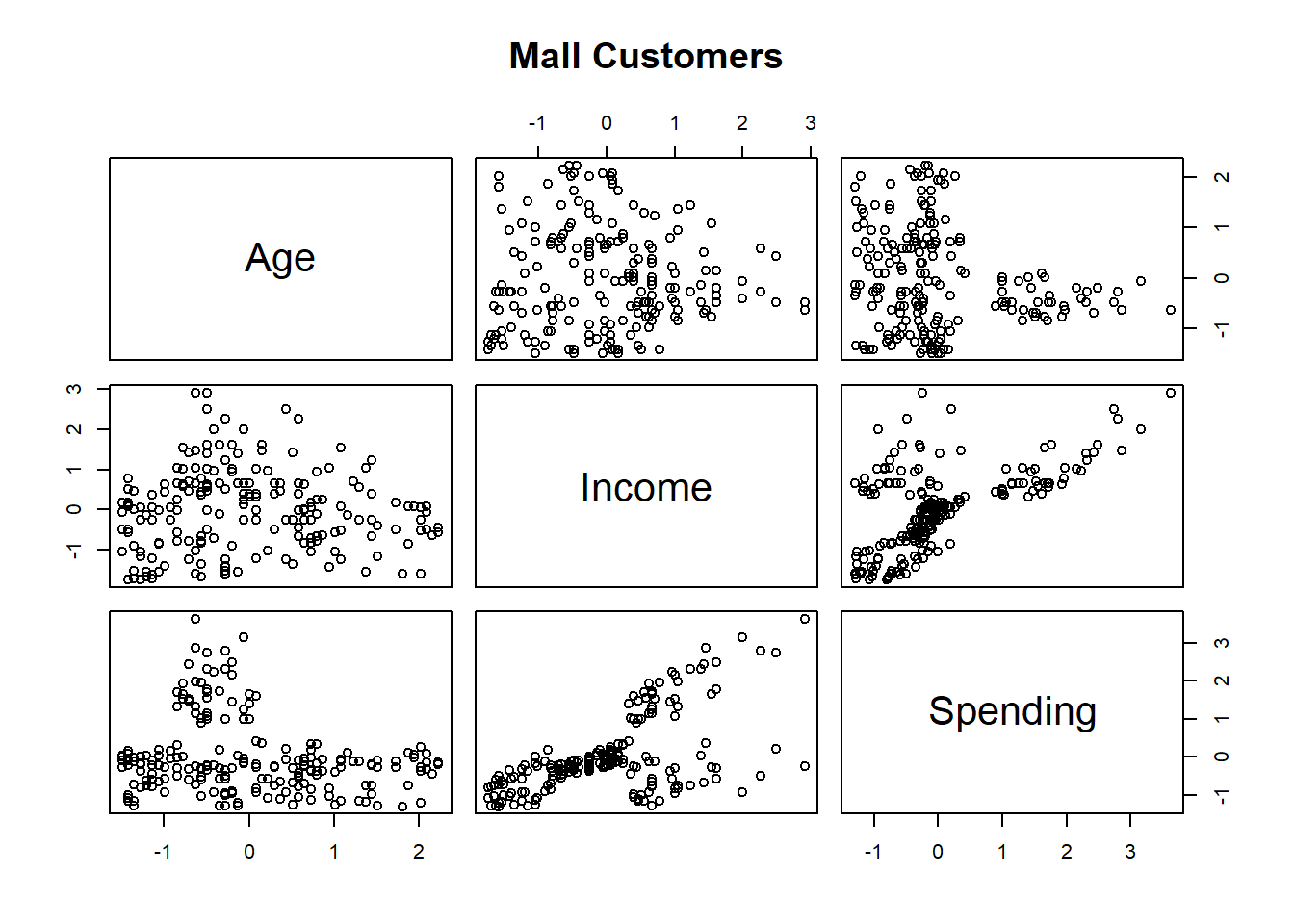
The scatter plot analysis reveals a roughly linear relationship between Income & Spending. In contrast, Age & Income do not exhibit a clear pattern, same is the case with Age & Spending.
Shifting our perspective from a strictly statistical to a more qualitative interpretation, we observe that individuals in the younger to middle-aged brackets display a wide spectrum of spending behaviors, from conservative to liberal. Conversely, the senior demographic is characterized predominantly by a tendency towards lower spending levels.
This variation in consumer behavior, particularly the nuanced differences within age groups, sets the stage for using fuzzy logic in modelling. Fuzzy logic excels at capturing the vagueness and complexity inherent in human language and decision-making processes. We can devise fuzzy logic systems to representing the gradual transitions observed in real-world scenarios, such as the gradual decrease in spending with age.
Code
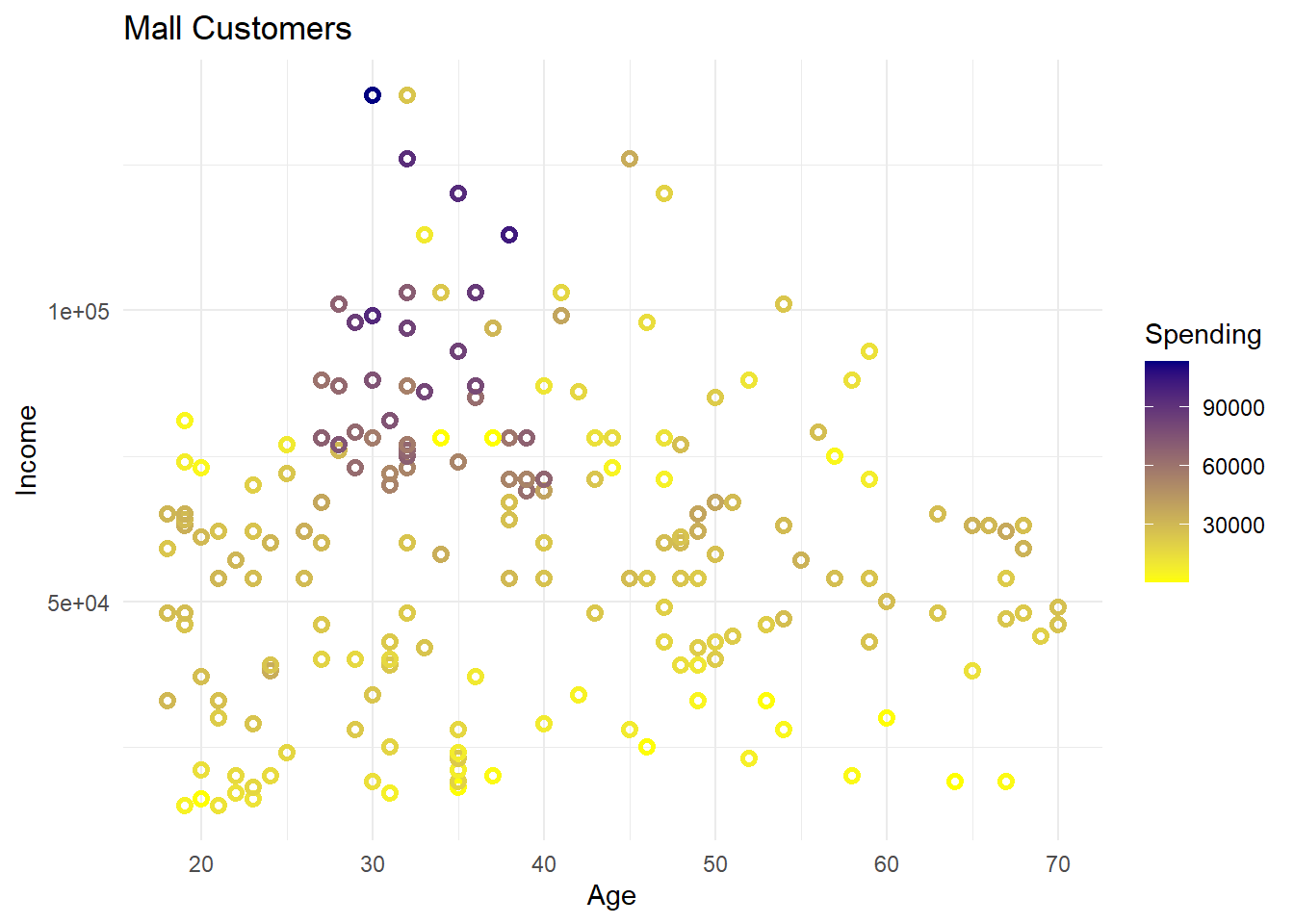
library(ggplot2)ggplot(data, aes(x=Age, y=Income))+geom_point(aes(color=Spending),shape=21,stroke=1.5)+scale_color_gradient(low='yellow',high='navy',name='Spending')+labs(x ='Age', y ='Income', title ='Mall Customers')+theme_minimal()
In this scatter plot, we observed the relationship between Age, Income and Spending. The plot uses colors to represent the amount of Spending, with the scale indicating higher spending in purple and lower spending in yellow.
The color gradient indicates that higher spending is more frequently observed among customers with higher incomes, regardless of age. The upper section of the plot, which corresponds to higher incomes, has more instances of purple dots. This suggests that within this group of mall customers, higher earners are likely to spend more.
There’s a cluster of higher spenders in the mid-income range (around 50,000 to 80,000) who are roughly between 20 to 40 years old. On the other hand, the lower and middle-income brackets show more variability in spending, not strongly correlated with age.
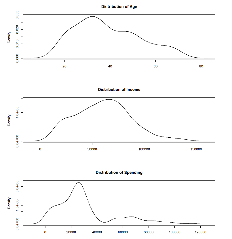
The distribution of Age appears to be slightly right-skewed, indicating a larger number of younger customers compared to older ones. The distribution tails off as age increases, with fewer customers in the older age brackets.
The distribution of Income is bimodal, indicating two prevalent groups within the data. The first peak occurs in the lower income bracket, while the second peak is in the higher income bracket.
The distribution of Spending is right-skewed, with a sharp peak in the lower spending bracket. This suggests that a majority of customers spend at lower levels, with fewer customers spending more. There’s a long tail extending towards higher spending amounts, which indicates that while there are customers who spend a lot, they are relatively few compared to the majority who spend less.
K-Means Clustering
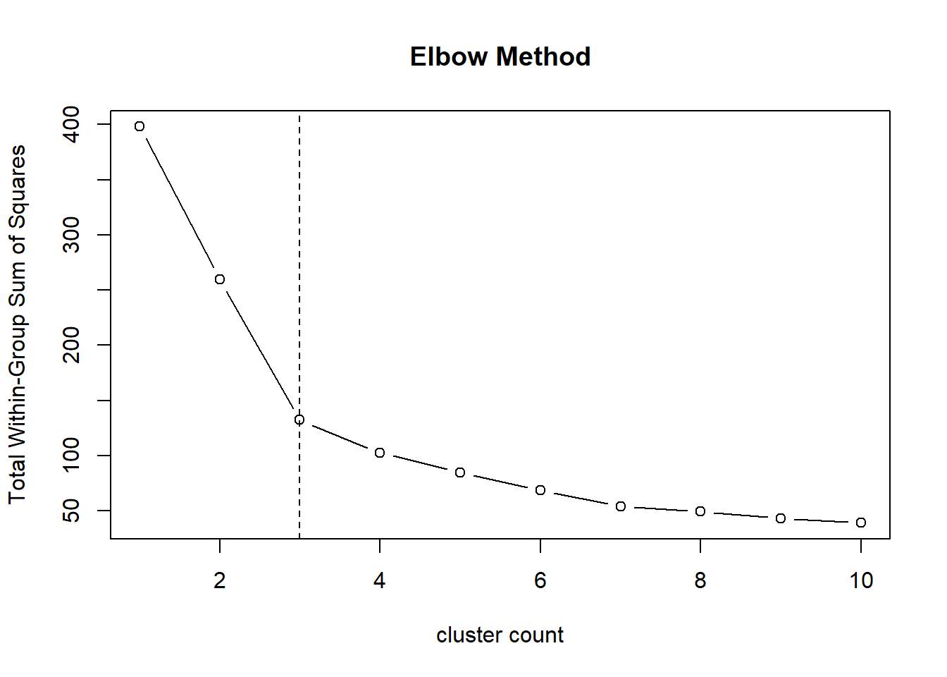
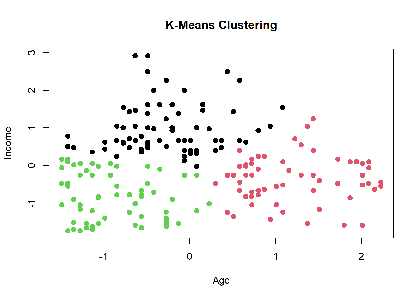
Let’s build a K-means model. First, in order to determine the optimal number of cluster centers, we use the Elbow Method, wherein we make a lot of models & compare their performance.
Code
set.seed(2023)tot.withinss =numeric()for(i in1:10) {set.seed(6) tot.withinss[i] =kmeans(df[,c('Age','Income')], i)$tot.withinss}plot(1:10, tot.withinss, type="b", xlab="cluster count",ylab="Total Within-Group Sum of Squares",main="Elbow Method")abline(v=3, lty=2) # let's consider k = 3
The ‘elbow’ of the plot is the point after which the decrease in Total Within-Group Sum of Squares starts diminishing. In this graph, the elbow appears to be at the cluster count of 3, marked by the dashed vertical line. This suggests that increasing the number of clusters beyond 3 leads to a lesser gain in the performance metric (Total WSS). Choosing 3 clusters may be the most reasonable choice based on this method, as it represents a balance between maximizing variance explained and minimizing the number of clusters.
Let’s consider a customer aged 35 years with an annual income of Rs 50,000.
Code
age =35income =50000scaled.age = (age - data.mean['Age'])/data.sd['Age']scaled.income = (income - data.mean['Income'])/data.sd['Income']newdata =data.frame(Age = scaled.age, Income = scaled.income)d1 =sum((kmeans$centers[1,] - newdata)^2) # dist from first centriodd2 =sum((kmeans$centers[2,] - newdata)^2) # dist from second centriodd3 =sum((kmeans$centers[3,] - newdata)^2) # dist from third centriodd =which.min(c(d1, d2, d3))cat('Input belongs to cluster number',d,'with centers:',kmeans$centers[d,])
Input belongs to cluster number 3 with centers: -0.8725537 -0.8288562
Code
# creating a new data frame to avoid disturbing entire structuredf2 = dfdf2$centers = kmeans$cluster # store clusters# reverse scaling and calculate average spending of that clusterpred =mean(df2$Spending[df2$centers==d]*data.sd['Spending'] + data.mean['Spending'])cat('Spending Output =', round(pred,2))
Spending Output = 21295.16
Fuzzy C-Means Clustering
Let’s build a Fuzzy Clustering Model using the fcm() function from the ppclust package, and it’s functionalities.
# the first data point belongs to cluster 1 with 0.813 membership# Initial cluster prototypesres.fcm$v0
                 Age      Income
Cluster 1 -0.4903713 -0.02132138
Cluster 2  1.5140661 -1.16353796
Cluster 3  1.0845438  1.53970795
Code
# Final cluster prototypesres.fcm$v
                 Age     Income
Cluster 1 -0.8288397 -0.9486545
Cluster 2  1.2051475 -0.2941141
Cluster 3 -0.3485579  0.8763321
In order to find the optimal solution, we can consider different starting points for the function fcm() by using the nstart argument. When we specify multiple starts, we can fix either the initial cluster prototypes (fixcent argument) or the initial membership degrees (fixmemb argument). Using best.start, iter & func.val we can see which among the multiple starts was the optimal one.
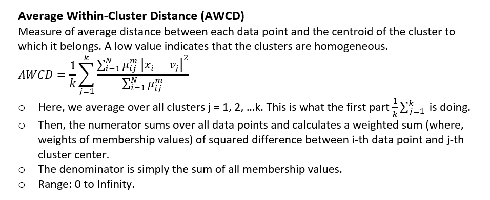
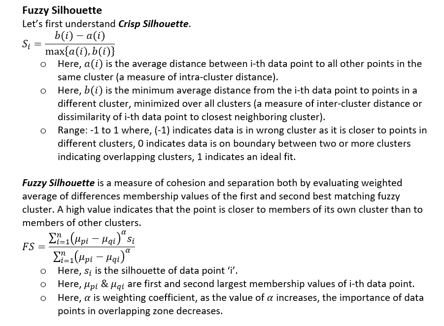
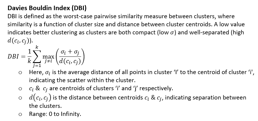
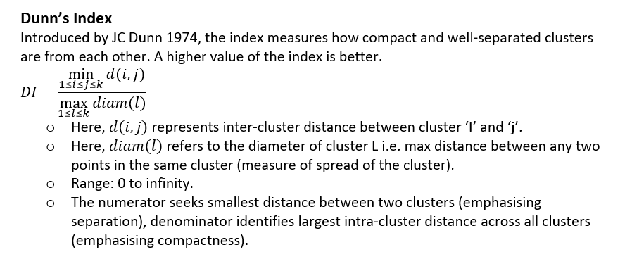
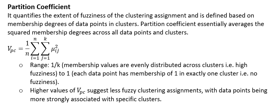
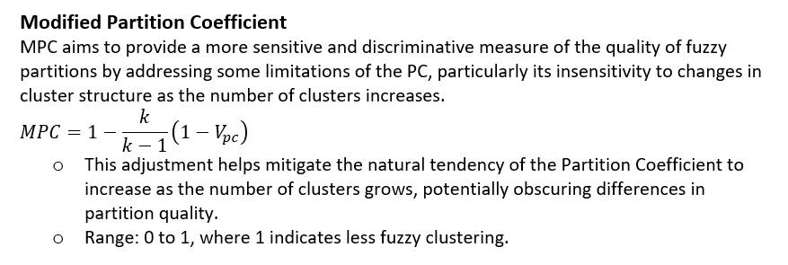
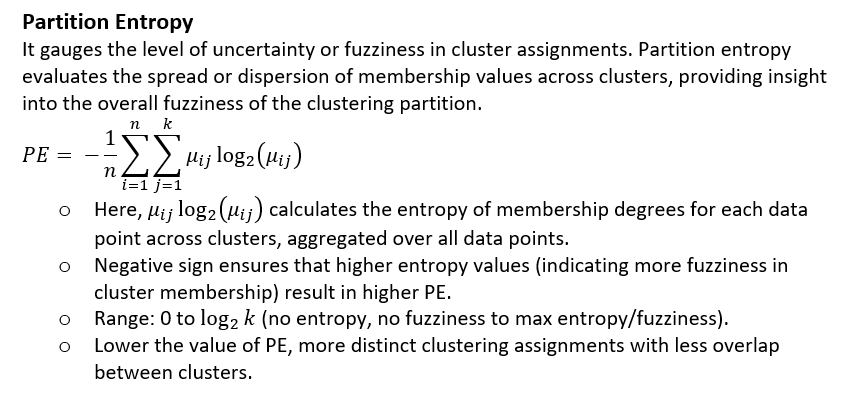
Let’s evaluate how well our clustering algorithm has performed by calculating some validity indexes. Since Clustering is an unsupervised learning analysis which does not use any external information, internal indexes are used to validate the clustering results. The aim of clustering algorithms is to make clusters that are homogeneous (i.e. similar points are grouped together - property called cohesion) and clusters are not overlapping & distinct (property called separation). To assess these properties, various internal validity indexes can be used:
Code
# let's run our clustering algorithm firstset.seed(2023)res.fcm =fcm(x = df[,c('Age','Income')], centers =3)# store crisp clusterscluster = res.fcm$cluster# using package fclustres.fcm2 =ppclust2(res.fcm, 'fclust')
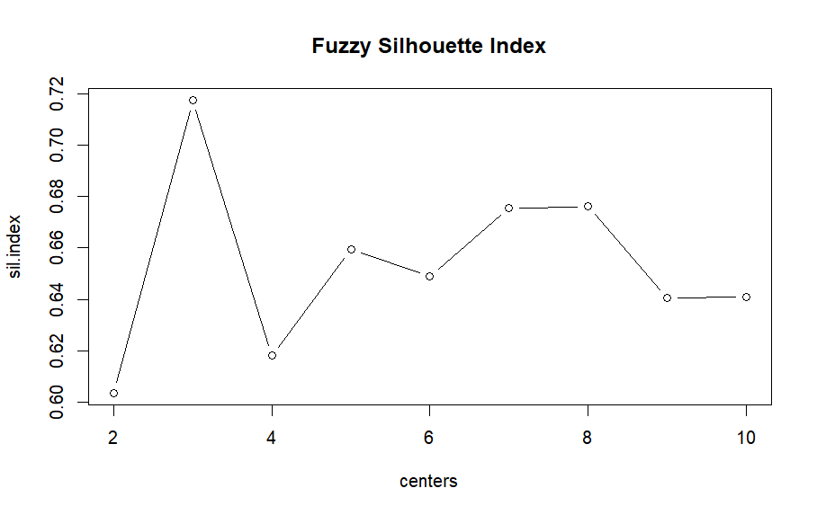
The highest Fuzzy Silhouette Index occurs at 3 centers, with a value above 0.70, suggesting that the data is best partitioned into 3 clusters. As the number of centers increases or decreases from 4, the Silhouette index generally decreases. This suggests that there is less clarity in cluster assignments, and data points might be less appropriately matched to their own clusters.
However this article will proceed with the analysis using 6 centers. This will later allow us to delve into the nuances of fuzzy logic, showcasing its flexibility and potential for fine-tuning the granularity of our analysis.
Code
c =6# number of centersfcm <-fcm(x = df[,c('Age','Income')], centers = c)
Code
library(ggplot2)ggplot(df, aes(x=Income, y=Age))+geom_point(aes(color=apply(fcm$u,1,max)),shape=21,stroke=1.5)+scale_color_gradient(low='yellow',high='purple',name='Membership Value',limits=c(0,1),breaks=seq(0,1,0.25))+labs(x ='Income', y ='Age', title ='Fuzzy Clustering')+theme_minimal()+geom_point(data=as.data.frame(fcm$v), aes(x=Income,y=Age),color='black',size=3,shape=4,stroke=2)
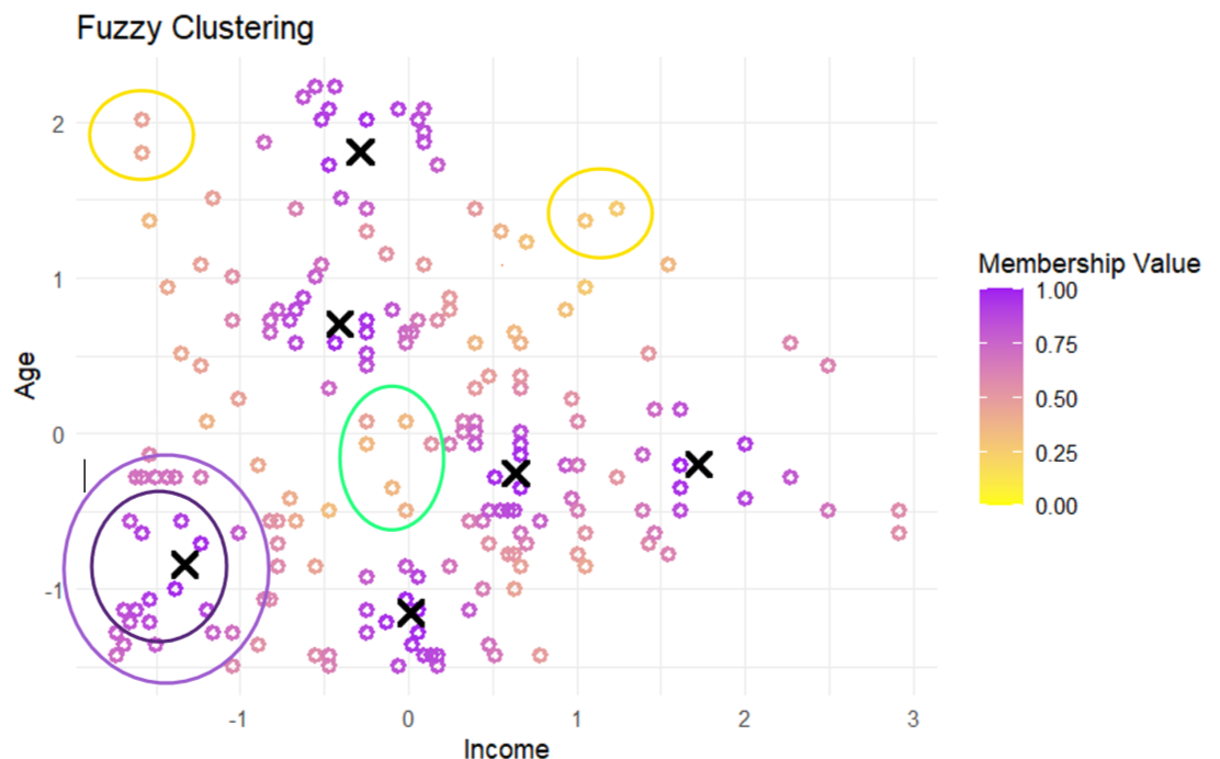
This scatter plot illustrates six clusters formed by a fuzzy clustering algorithm, marked by black ‘X’ symbols for the cluster centers. The color intensity of the points reflects their membership values, with darker colors indicating higher membership to the nearest cluster center. Points in the innermost areas show strong membership, while those further away show decreasing membership, evidenced by lighter colors.
Points within yellow circles have light shades, suggesting they are outliers with low membership to all clusters. Points within the green circle, displaying shades of orange, are positioned close to multiple clusters, indicating shared membership and highlighting the fuzzy nature of the cluster boundaries.
Now, we will use Gaussian Approximation to form our fuzzy sets for Age and Income.
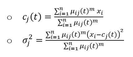
We use the cluster centers as the ‘mu’ and evaluate the ‘sigma’ parameter for our Gaussian distribution as shown above.
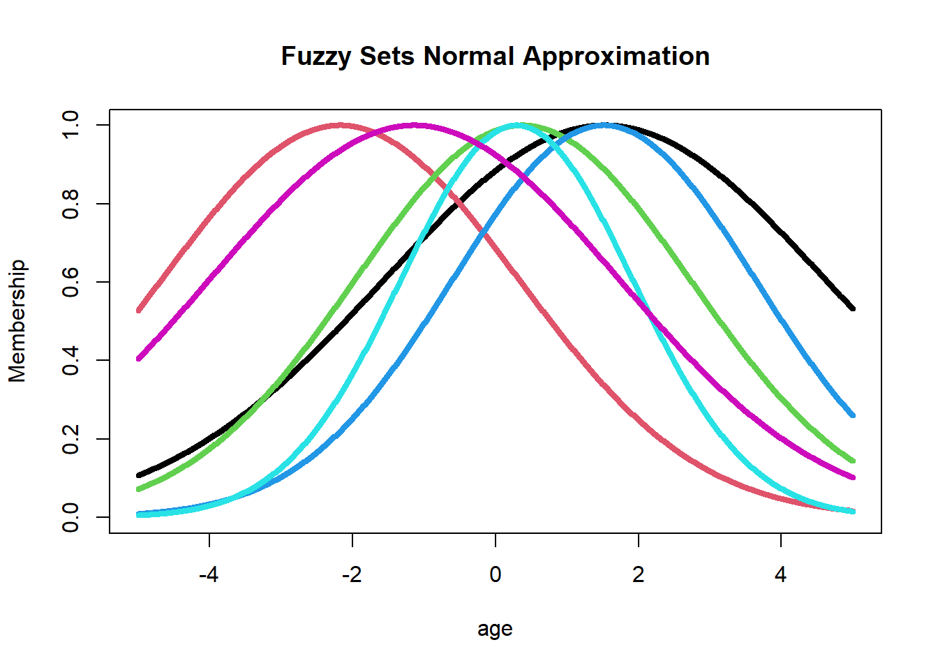
# let's define our domainage =seq(-5,5,0.01)# store the respective gaussian distributionsd =list()for(i in1:c) d[[i]] =gaussian(age,c_j[i],sigma_j[i]^0.5) # plot themplot(age, d[[1]], type='l', ylim=c(0,1),col=1,lwd=4,ylab ='Membership',main='Fuzzy Sets Normal Approximation')for(i in2:c) lines(age, d[[i]], col=i, lwd=4)
These Gaussian approximations give us fuzzy sets for our input variables ‘Age’ and ‘Income’. However, a lot of these fuzzy sets are overlapping. So, it is better to merge the ones which are similar. Now this begs the question on how do we determine which sets are similar and then how do we merge them!
Merging Similar Sets
The first method is to Merge based on Similarity using methods like Jaccard Similarity between the fuzzy sets. For this we calculate a matrix of similarity scores between each pair of these fuzzy sets. Then we iteratively merge the ones with the highest values. This method has two drawbacks - (a) we need to decide on a threshold to stop merging and (b) its computationally expensive in case of large number of sets.
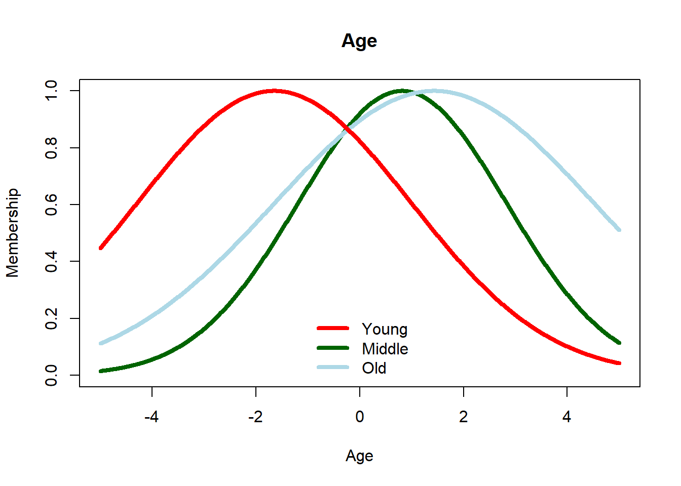
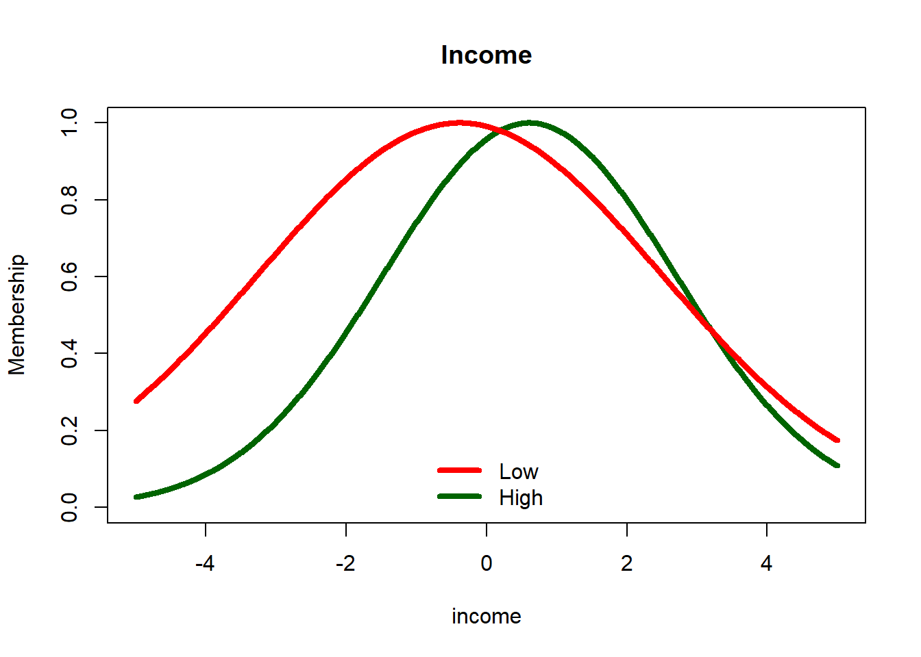
Another approach is to Merge in the Parameter Space. The idea here is to perform clustering in the parameter space (imagine a co-ordinate system with mu and sigma). So from 6 values of \(\mu\) and \(\sigma^2\), we can make clusters representing the similar ones. Following this idea, we can create 3 clusters/fuzzy sets representing Age and 2 sets for Income.
Code
# merging using fuzzy-clustering in parameter space for agefcm.p =fcm(data.frame(c_j,sigma_j),3)age.young =function(x) gaussian(x,fcm.p$v[,'c_j'][1], fcm.p$v[,'sigma_j'][1]^0.5)age.middle =function(x) gaussian(x,fcm.p$v[,'c_j'][2], fcm.p$v[,'sigma_j'][2]^0.5)age.old =function(x) gaussian(x,fcm.p$v[,'c_j'][3], fcm.p$v[,'sigma_j'][3]^0.5)plot(age, age.middle(age), type='l', ylim=c(0,1),col='darkgreen',lwd=4,main='Age',ylab='Membership',xlab='Age')lines(age, age.old(age), type='l', col='lightblue',lwd=4)lines(age, age.young(age), type='l', col='red',lwd=4)legend('bottom',c('Young','Middle','Old'),lwd=4,bty='n',lty=1,col=c('red','darkgreen','lightblue'))
Code
# merging using fuzzy-clustering in parameter space for incomeincome =seq(-5, 5, 0.01)fcm.p2 =fcm(data.frame(c_j,sigma_j),2)income.low =function(x) gaussian(x,fcm.p2$v[,'c_j'][2], fcm.p2$v[,'sigma_j'][2]^0.5)income.high =function(x) gaussian(x,fcm.p2$v[,'c_j'][1], fcm.p2$v[,'sigma_j'][1]^0.5)plot(income, income.high(income), type='l', ylim=c(0,1),col='darkgreen',lwd=4, main='Income',ylab='Membership')lines(income, income.low(income), type='l', col='red',lwd=4)legend('bottom',c('Low','High'),lwd=4,bty='n',lty=1,col=c('red','darkgreen'))
Now let’s create our Output Fuzzy set for Spending.
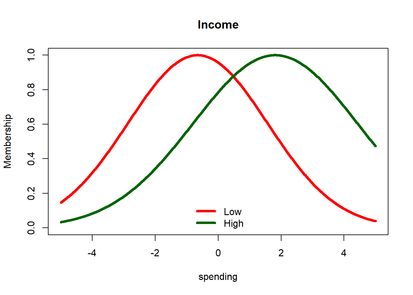
Looking at the summary of spending values (scaled ones), we can see that the values range from -1.3049 to 3.633 with a mean of 0. So here, we split it about the mean into Low and High. Thus, the mean of for low spending with the average of (-1.3049, 0) and mean of high spending is average of (0, 3.633). The sigma parameter is evaluated as : 2 + ( 0 + 1.3049)/6 and 2 + (3.633 -0)/6. These are parameter values are chosen arbitrarily for now.
Code
# summary(df$Spending)# guassian for low spending -> mu = -0.65, sigma = 2.2167# guassian for high spending -> mu = 1.815, sigma = 2.605spending =seq(-5, 5, 0.01)spend.low =function(x) gaussian(x, -0.65, 2.2167)spend.high =function(x) gaussian(x, 1.815, 2.605)plot(spending, spend.low(spending), type='l', ylim=c(0,1),col='red',lwd=4, main='Income',ylab='Membership')lines(spending, spend.high(spending), type='l', col='darkgreen',lwd=4)legend('bottom',c('Low','High'),col=c('red','darkgreen'),lwd=4,bty='n',lty=1)
Fuzzy Logic System
We will construct a Fuzzy Logic System that includes two input variables: ‘Age’ and ‘Income.’ The ‘Age’ variable encompasses three linguistic terms—‘Young,’ ‘Middle,’ and ‘Old,’ while ‘Income’ is categorized as either ‘Low’ or ‘High.’ The output variable, ‘Spending,’ is similarly bifurcated into ‘Low’ and ‘High’ categories, with the membership functions for these determined from previous analysis.
Let’s define our fuzzy inference rules:
IF Age is Young OR Income is Low THEN Spending is Low
IF Age is Old THEN Spending is Low
IF Age is Middle AND Income is High THEN Spending is High
These rules are formulated to capture the nuances of consumer spending behavior, based on the combined effects of age and income on spending patterns. They serve as the basis for decision-making in our Fuzzy Logic System, enabling it to process input information and deduce the appropriate spending category.
Code
w1 =min(age.young(scaled.age), income.low(scaled.income))w2 =age.old(scaled.age)w3 =max(age.middle(scaled.age), income.high(scaled.income))cat('Firing strength of Rule 1 =',w1,', of Rule 2 =',w2,'and of Rule 3 =',w3)
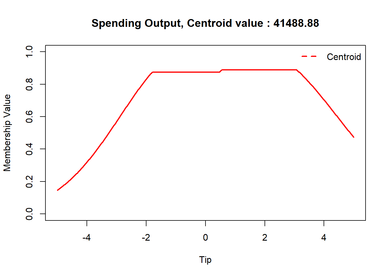
Firing strength of Rule 1 = 0.8739534 , of Rule 2 = 0.8562308 and of Rule 3 = 0.8883313
Code
# shape of output fuzzy set final =pmax(pmin(w1,spend.low(spending)), pmin(w2,spend.low(spending)),pmin(w3,spend.high(spending)))# centroid defuzzificationcentroid_value =round(sum(spending*final)/sum(final),3)centroid_value =round(centroid_value*data.sd['Spending'] + data.mean['Spending'],2)plot(spending, final, type='l', col='red', xlab='Tip', ylab='Membership Value', lwd=2, ylim=c(0, 1),main=paste('Spending Output, Centroid value :',centroid_value))abline(v=centroid_value, lty=2, lwd=2, col='red')legend('topright',c('Centroid'),lty=2,lwd=2,col='red',bty='n')
Experimentation
To compare the performance of our FCM-based Fuzzy logic system, let’s use Linear Regression and Random Forest models alongside K-means.
Code
# linear regressionfit =lm(Spending ~ Age + Income, data= data)# Spending = 11860 - 311.2*Age + 0.5068*Income# where, error ~ N(0, 18190)# adjusted R-square = 36.99%pred.lm =predict(fit, data.frame(Age =35, Income =50000))# decision tree / random forestlibrary(randomForest)set.seed(2023)rf =randomForest(Spending ~ Age + Income, data = data)# 500 trees, % Var explained = 48.34%pred.rf =predict(rf, data.frame(Age =35, Income =50000))
Let’s summarize our existing data. Based on Age, we calculate the average income and spending.
Code
library(dplyr)mean((data %>%filter(Age <40& Age >30))[,'Income'])mean((data %>%filter(Age <40& Age >30))[,'Spending'])mean((data %>%filter(Age ==35))[,'Income'])mean((data %>%filter(Age ==35))[,'Spending'])
Age
Avg. Income
Avg. Spending
30 to 40
69,400
41, 680
35
46,667
34,100
Results
Model
Predicted Spending (approx.)
FCM based Fuzzy Logic System (centroid)
41, 500
Linear Regression
26, 300
Random Forest
25, 100
K-Means Clustering (cluster-center)
21, 300
The analysis of the data and model predictions reveals critical insights into the spending patterns of our customer base, specifically targeting the age group of 30-40 years. The observed average income for this demographic is $ 69, 400 approx with an average spending of $ 41, 700. However, a more detailed look at customers aged 35 shows an average income of 46, 700 with an approx average spending of 34, 100.
When comparing these real world observations with the predictions made by our predictive models, we see a consistent underestimation of spending. The closest prediction to the actual average spending comes from our FCM-based Fuzzy logic system, with an estimate of approx $ 41, 500. The other models predict a lot lower spending, with estimates ranging from $21, 300 to $26, 300.
This consistent under-performance, as indicated by both the adjusted R-square and percentage of variance explained, suggests these models may not be capturing all nuances of our customer base. The discrepancy between model’s predictions and the actual spending figures could be atttributed to various factors, such as the model’s inability to capture the overlapping nature and behavior of our customers based on different variables. This is where our FCM-based Fuzzy logic system outperforms as it can adapt better to uncertain and overlapping data.
Going forward, we can incorporate more comprehensive data, exploring alternative modelling techniques that can capture the complexity of consumer spending. We can also explore other fuzzy rules and systems to possibly produce more refined results.
Research Papers
These are a few research papers you can explore and enhance your understanding in the realm of Fuzzy Logic and Clustering:
(link) Customer Segmentation Through Fuzzy C-Means & Fuzzy RFM Method
(link) A New Fuzzy Set Merging Technique Using Inclusion-Based Fuzzy Clustering
(link) A New Cluster Validity Index For The Fuzzy C-Mean
(link) A Fuzzy Extension Of The Silhouette Width Criterion
(link) A Possibilistic Fuzzy C-Means Clustering Algorithm
(link) TSK-Fuzzy Modeling Based On spl_epsiv-Insensitive Learning
Conclusion
This article is part of a comprehensive series on Fuzzy Logic and Systems using R, laying the groundwork for understanding advanced concepts and applications in this field.
For further exploration, you can access other articles in this series:
The work in this article is inspired by the teachings of my Professors at the University of Nottingham. Their guidance and expertise have greatly influenced the content and direction of these articles. For further insights into their research and contributions, you can visit their University of Nottingham profiles:
These articles aim to delve deeper into Fuzzy Logic concepts and their practical implementations, building upon the foundation laid by our esteemed professors. Stay tuned for more valuable insights and applications in this exciting field.