Introduction to Fuzzy Logic in R

Author

Kunal Choudhary

Published

November 5, 2023

ABSTRACT

This article is aimed towards introducing Fuzzy Sets and Logic. We will code from scratch & explore some in-built packages for implementation in R. By understanding and applying fuzzy logic, we can enhance decision-making processes in complex, uncertain environments such as finance, healthcare, and engineering.

Introduction

Uncertainty plays a fundamental role in our quest for knowledge, from the unpredictability of events to the fuzziness of real-world phenomena. Historically, our understanding and handling of uncertainty have evolved, moving from viewing it as a flaw to embracing it as an inherent part of scientific inquiry and decision-making. This shift became particularly evident with the advent of statistical methods and quantum mechanics in the 20th century, laying the groundwork for modern approaches to dealing with ambiguity.

In our daily lives and scientific endeavors, we often encounter situations that cannot be neatly categorized into binary outcomes of true or false. Recognizing this, fuzzy logic offers a nuanced way to interpret these uncertainties. Unlike Boolean logic, which confines us to a black-and-white view of the world, fuzzy logic introduces shades of grey by allowing truth values to range between 0 and 1. This approach is particularly powerful in fields like computer and data science, where it helps to model complex systems, make decisions under uncertainty, and process imprecise information.

Fuzzy sets, an extension of classical logic, allow elements to belong to a set with varying degrees of membership, reflecting the real-world complexity where categorical boundaries are often blurred. The Sorites paradox, or the paradox of the heap, serves as a poignant illustration of this concept. It questions when a heap of sand ceases to be a heap as grains are removed one by one, highlighting the challenges of defining precise boundaries in natural language and phenomena. Fuzzy logic embraces this ambiguity, providing a framework to quantify and navigate the gradations between binary extremes.

As we delve into fuzzy logic and its applications, we’ll explore how this innovative approach enables us to better model and understand the nuanced reality around us, offering valuable tools for tackling complex problems in various domains, from healthcare to autonomous driving.

Fuzzy Logic vs. Probability

At first glance, fuzzy logic and probability theory share a common trait: both operate within the numeric range of [0, 1]. However, this similarity is superficial — probability quantifies the degree of randomness and fuzzy logic deals with the degrees of belongingness.

In probability theory, we quantify uncertainty in terms of randomness. For example, when tossing a coin, we assess the probability of outcomes (Heads or Tails) within a framework that anticipates uncertainty through the lens of chance.

Conversely, fuzzy logic introduces a nuanced perspective on belongingness. Consider human height, which may be categorized into sets such as “Tall,” “Average,” and “Short.” Unlike a probabilistic view, fuzzy logic allows us to assign a degree of membership to these sets, reflecting real-world ambiguity where categories are not strictly binary.

Classical Set vs. Fuzzy Set

A Classical Set, A = {x : 15 < x < 20} or explicitly as {16,17,18,19}, where elements either completely belong (100% or 1) or do not belong (0%) to the set A. This binary membership aligns with Boolean logic.
A Fuzzy Set, A = { (16, 0.6), (17, 0.9), (18, 0.8), (19,1) }, where each element has a degree of membership to set A. For instance, the number 16 belongs to A with a membership value of 0.6. This aligns with the essence of Multi-valued logic.

This distinction underscores the innovative approach of fuzzy logic in capturing the complexities and gradations inherent in real-world phenomena, a capability that traditional probabilistic methods cannot emulate as effectively.

Membership Functions

At the heart of applying fuzzy logic to real-world problems is the concept of membership functions. These functions translate the qualitative aspects of human reasoning and natural language into quantitative values, enabling machines to process and analyze complex, ambiguous information.

Common Membership functions are Triangular, Trapezoid and Gaussian. However, we can design custom membership functions to suit specific data characteristics or industry requirements. This customization process involves analyzing the dataset, understanding the context of the application, and experimenting with different function shapes to capture the inherent vagueness or ambiguity effectively.

Let’s see how we can define some of the common membership functions in R, coding from scratch.

Code

# For exploring the functions, we define a domain of [0, 100] - our values on the x-axis.
domain = seq(0, 100, 0.1)

Code

# Triangular(x; a,b,c) = 0           for x <= a & x >= c
#                      = (x-a)/(b-a) for a <= x <= b
#                      = (c-x)/(c-b) for b <= x <= c

triangle = function(x, a, b, c){
  ifelse(x <= a, 0, ifelse(x <= b, (x-a)/(b-a), ifelse(x <= c, (c-x)/(c-b), 0)))
}
plot(domain, triangle(domain, 25, 50, 75), col='navy', lwd=2, 
     xlab='x', ylab='Membership Value', main='Triangle Membership Function')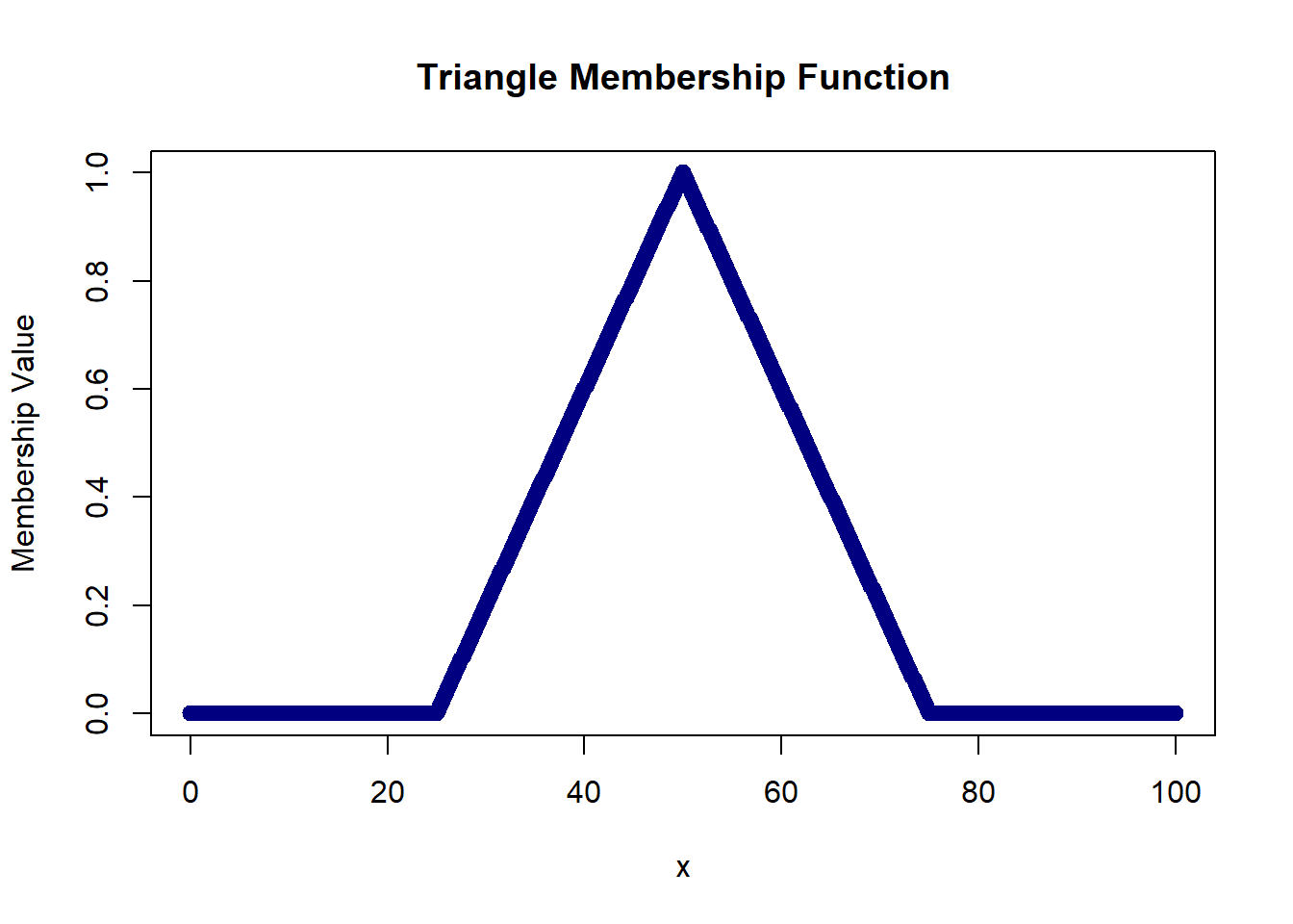

Left Open

Here, the ‘a’ and ‘b’ parameters are the same giving us a triangle that is open on the left side.

Right Open

Here, the ‘b’ and ‘c’ parameters are the same giving us a triangle that is open on the right side.

Code

par(mfrow=c(1,2))
plot(domain, triangle(domain, 0, 0, 50), col='navy', lwd=2, 
     xlab='x', ylab='Membership Value', main='Left Open Triangle')
plot(domain, triangle(domain, 50, 100, 100), col='navy', lwd=2,
     xlab='x', ylab='Membership Value', main='Right Open Triangle')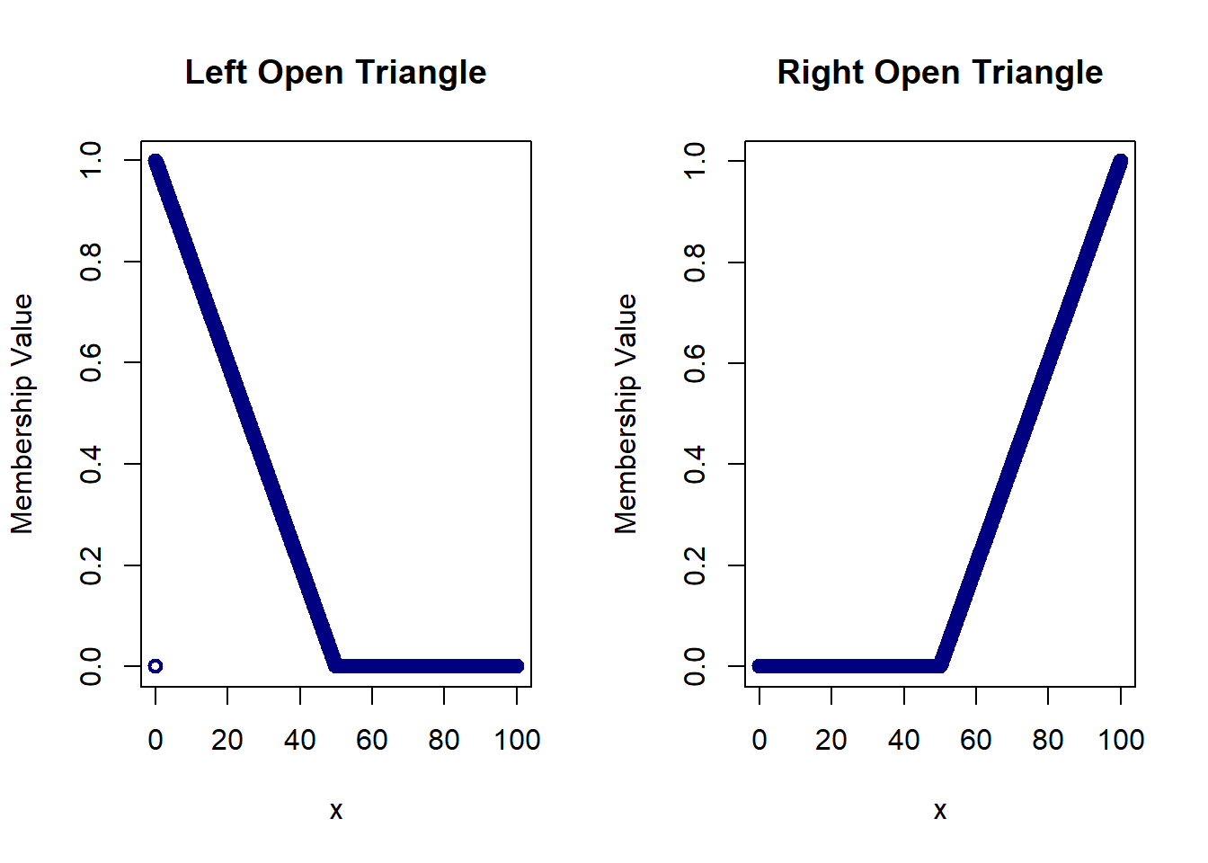

Code

# Trapezoid(x; a,b,c,d)= 0           for x <= a & x >= d
#                      = (x-a)/(b-a) for a <= x <= b
#                      = 1           for b <= x <= c
#                      = (d-x)/(d-c) for c <= x <= d

trapezoid = function(x, a, b, c, d){
  ifelse(x <= a, 0, ifelse(x <= b, (x-a)/(b-a), ifelse(x <= c, 1,
                                                       ifelse(x <= d, (d-x)/(d-c), 0))))
}
plot(domain, trapezoid(domain, 20, 40, 60, 80), col='navy', lwd=2,
     xlab='x', ylab='Membership Value', main='Trapezoid Membership Function')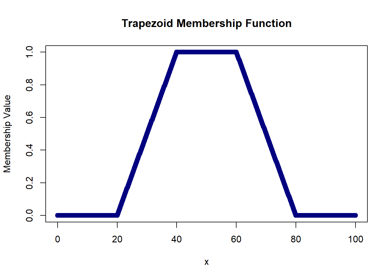

Code

# Gaussian = exp(-0.5*(x-mu)^2/sigma^2)
# where, mu is mean and sigma is standard deviation
gaussian = function(x, mu, sigma){
  exp(-0.5*(x-mu)^2/sigma^2)
}
plot(domain, gaussian(domain, 50, 10), col='navy', lwd=2, type='l',
     xlab='x', ylab='Membership Value', main='Gaussian Membership Function')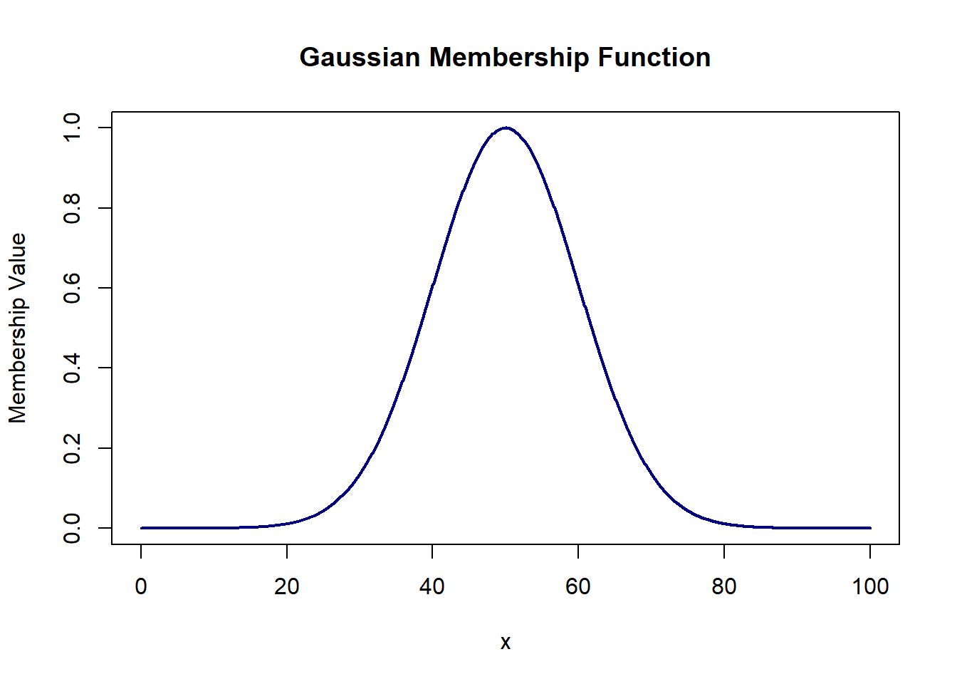

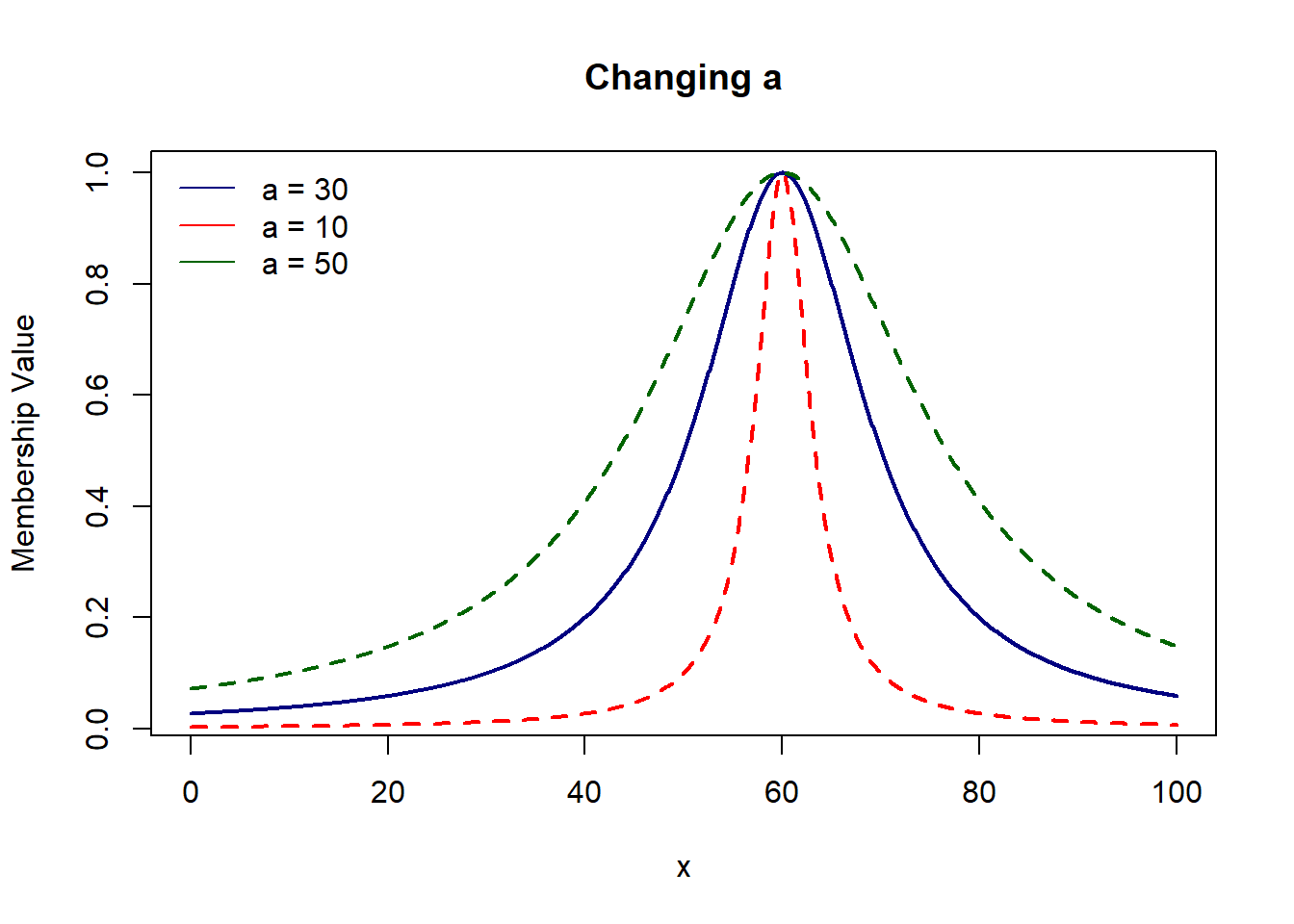
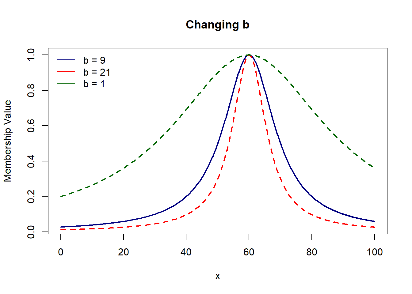
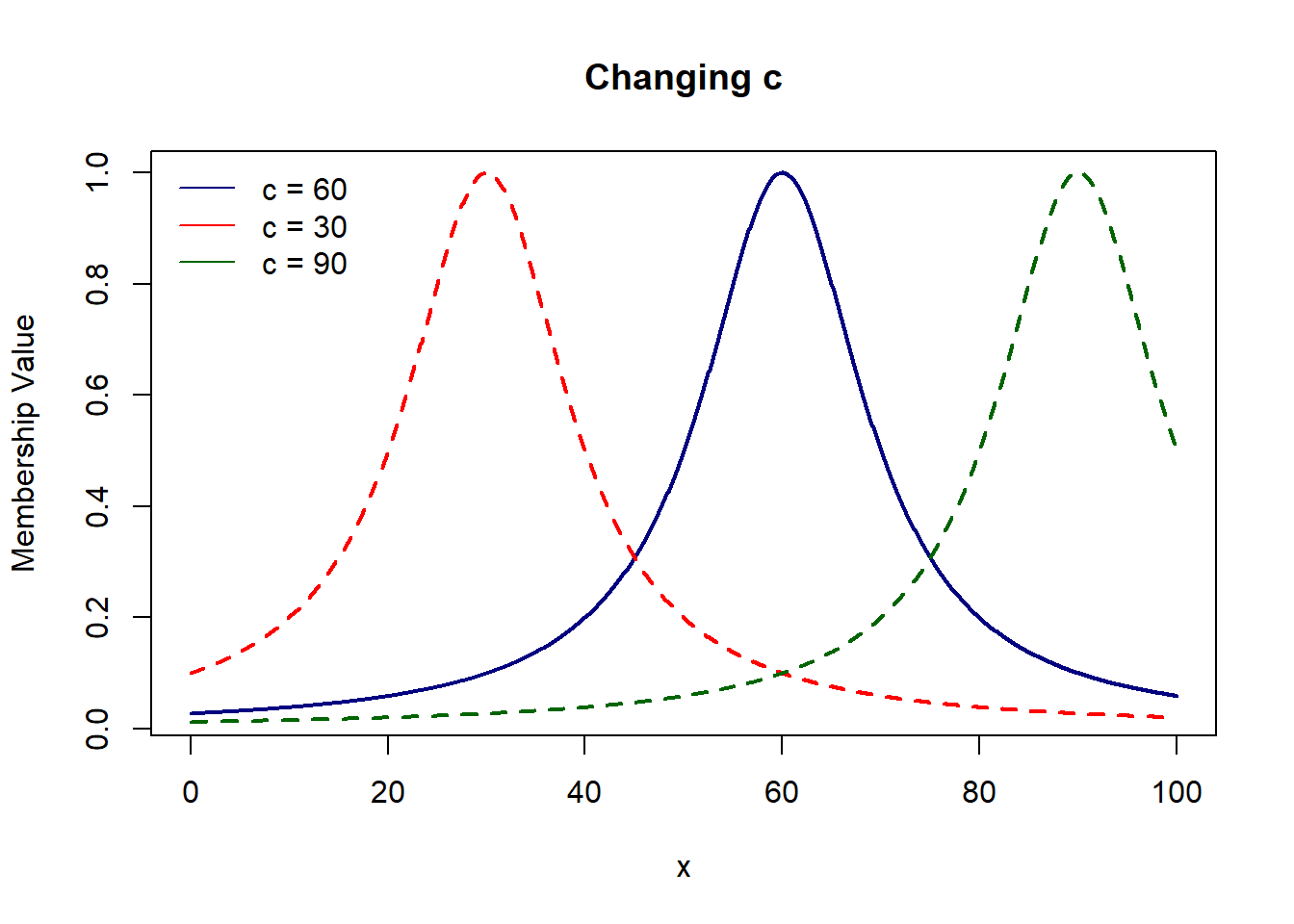
Code

# Gen Bell shaped = 1/(1+ mod[(x-c)/a]^2b)
# where, a = width, b = shape of curve, c = center

gen.bell = function(x, a, b, c){
  1/(1+ abs((x-c)/a)^2*b)
}
plot(domain, gen.bell(domain, 90, 9, 60), col='navy', lwd=2, type='l',
     xlab='x', ylab='Membership Value', main='Gen. Bell Shaped Membership Function')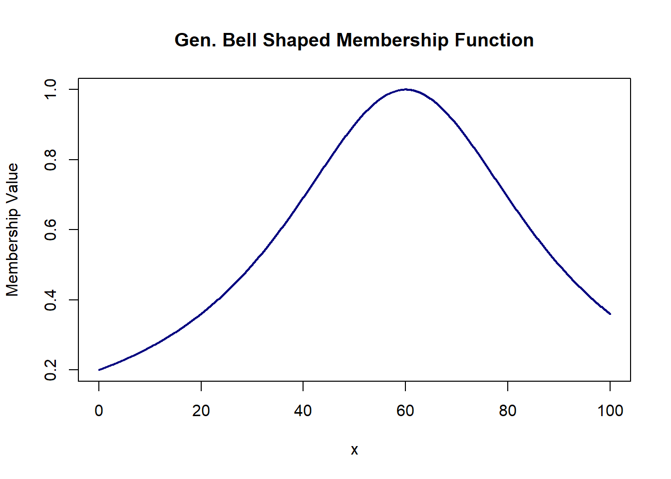

Changing parameter values

Code

# sigmoid = 1/(1 + exp(-a(x-c)))
sigmoid = function(x, a, c){ 1/(1 + exp(-a*(x-c))) }

plot(domain, sigmoid(domain, 0.5, 50), col='navy', lwd=2, type='l',
     xlab='x', ylab='Membership Value', main='Sigmoid Membership Function')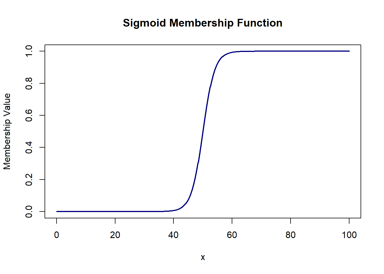

Code

# Left-Right =  f_left( (c-x)/a ) for x <= c
#            = f_right( (x-c)/b ) for x >= c

where, ‘c’ is the point where membership value is 1.
‘a’ is the width of region x <= c
‘b’ is the width of region x >= c
f_left and f_right are monotonically decreasing functions defined on [0, inf) with f_left(0) = f_right(0) = 1

Code

# example : f_left(u) = f_right(u) = exp(-mod(u)^3)
# it is not necessary that f_left and f_right are the same function
# (as taken in this example)
LR_function = function(x, a, b, c){
  ifelse(x <= c, exp(-abs((c-x)/a)^3), exp(-abs((x-c)/b)^3))
}
plot(domain, LR_function(domain, 40, 10, 70), col='navy', lwd=2, type='l',
     xlab='x', ylab='Membership Value', main='Left-Right Membership Function')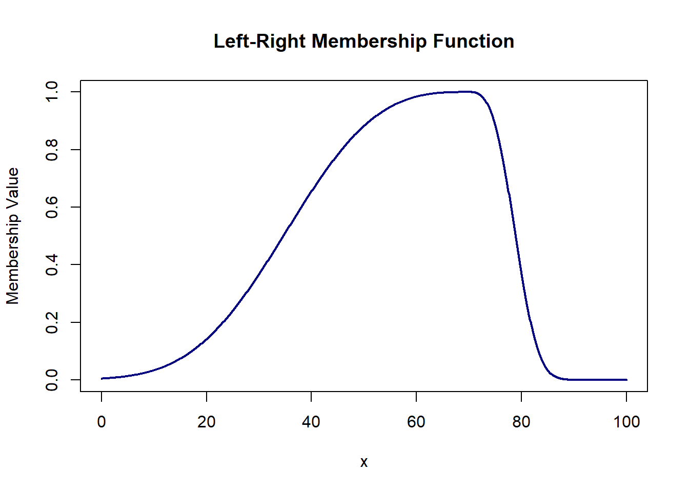

We can define the Pi-Shaped membership function using 2 or 4 parameters.

2 Parameter Pi-Shaped

This function has a membership value 1 at point ‘a’, 0.5 at a +/- b. The Pi function decreases toward zero asymptotically as we move away from ‘a’.

Code

# pi-shaped_2 = 1/(1 + (x-a)^2/b^2) 
pi_shaped2 = function(x, a, b){ 1/(1 + (x-a)^2/b^2) }

plot(domain, pi_shaped2(domain, 35, 25), col='navy', lwd=2, type='l',
     xlab='x', ylab='Membership Value', main='Pi-Shaped Membership Function')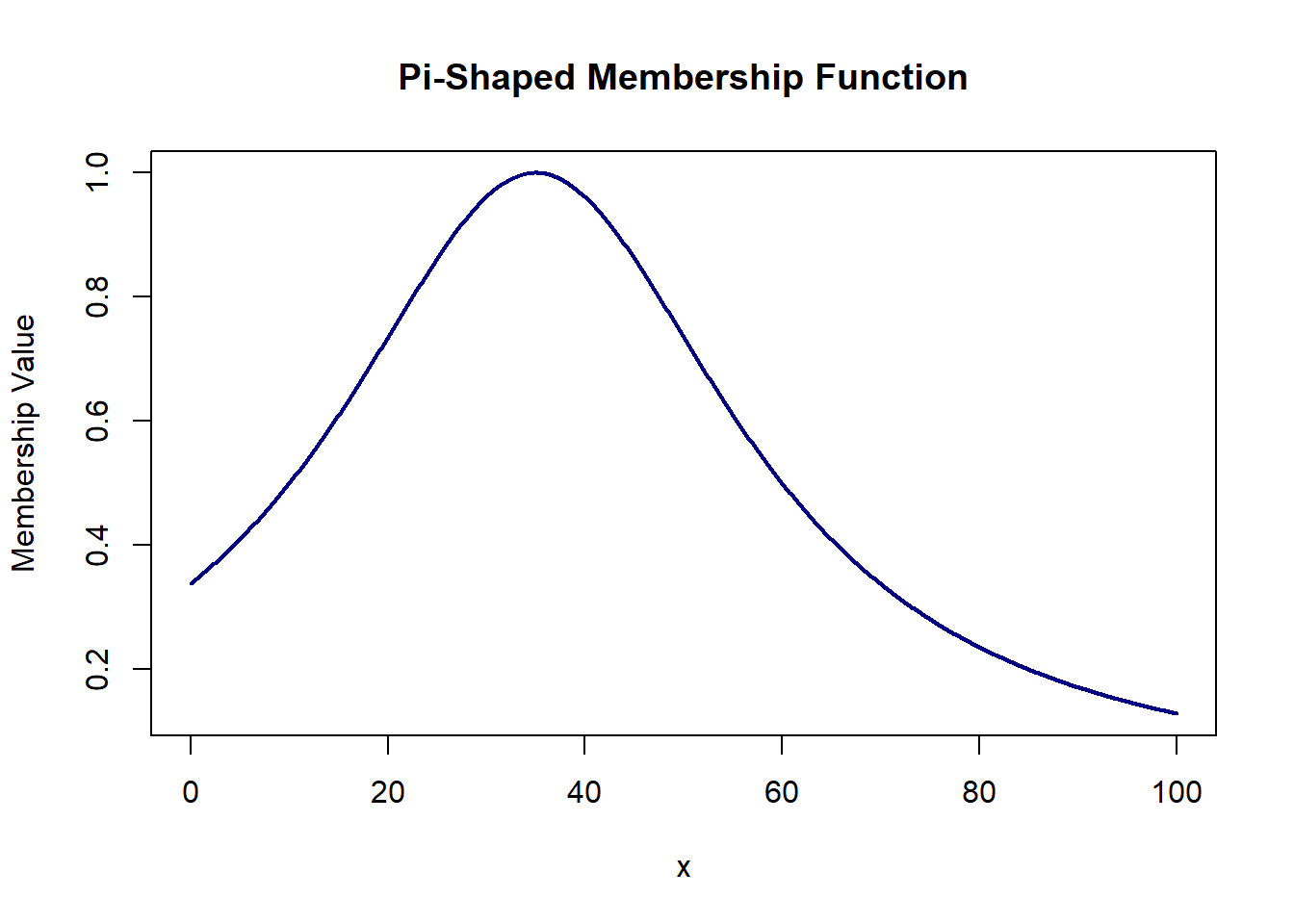

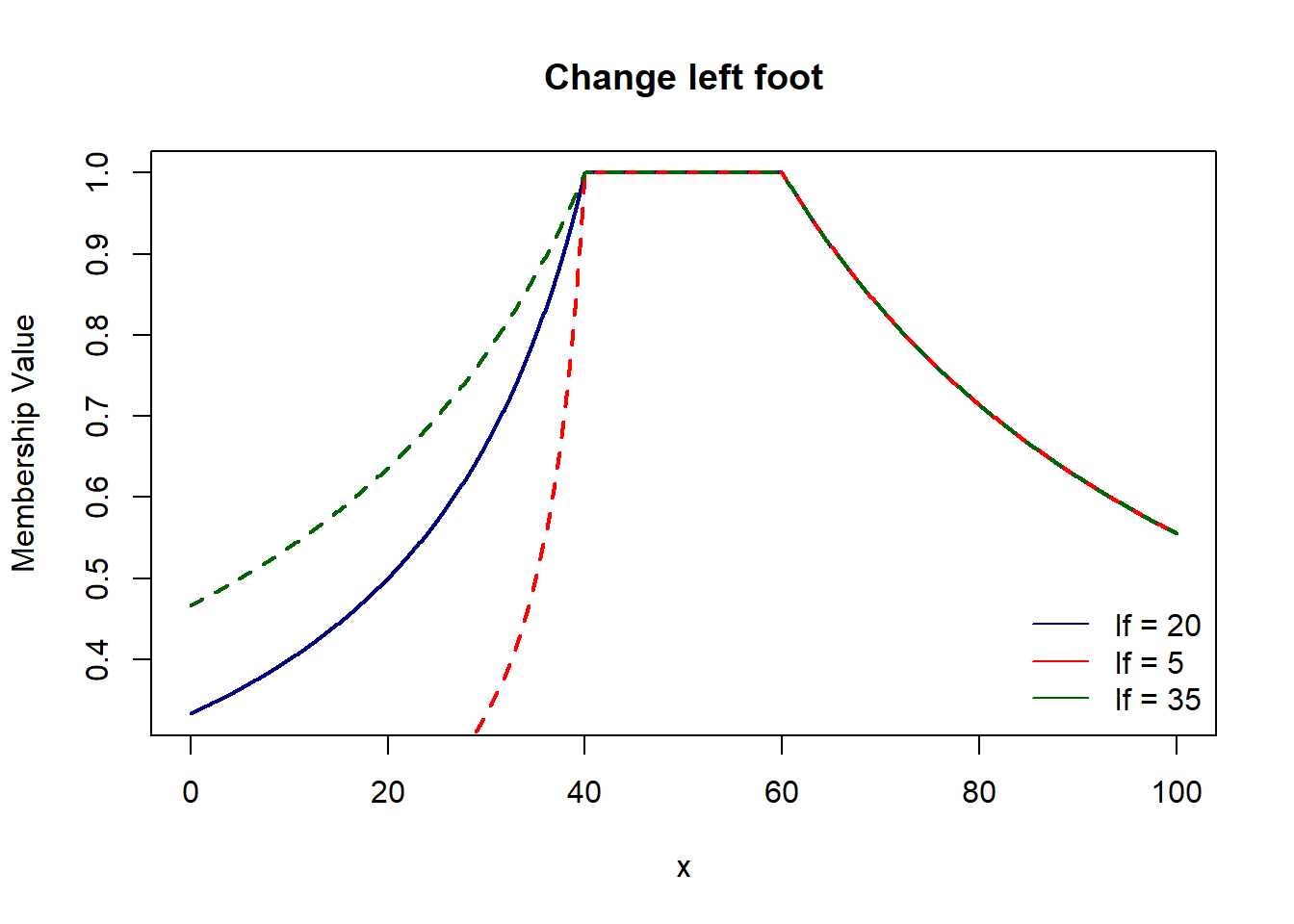
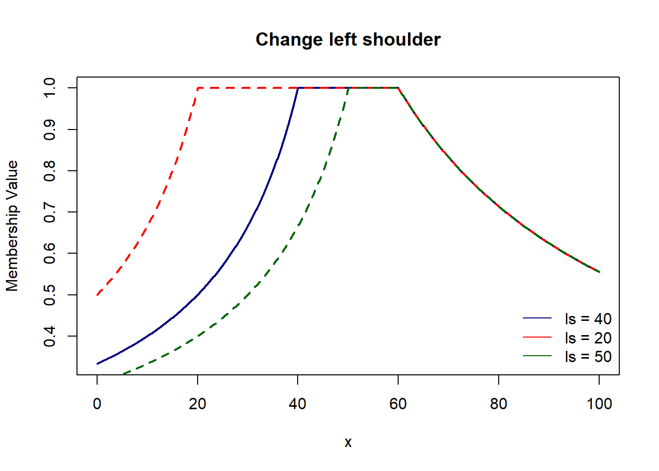
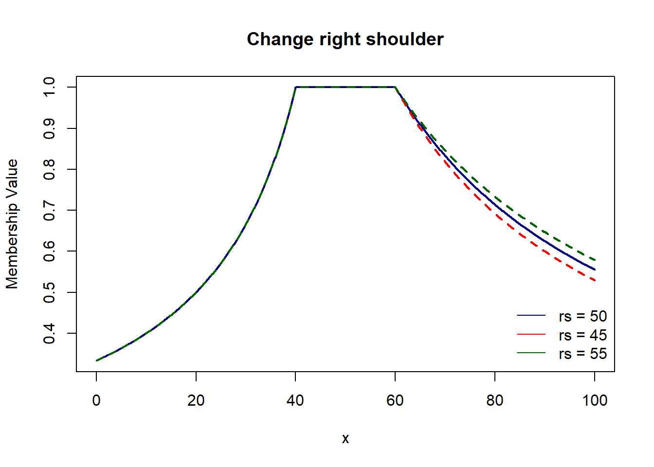
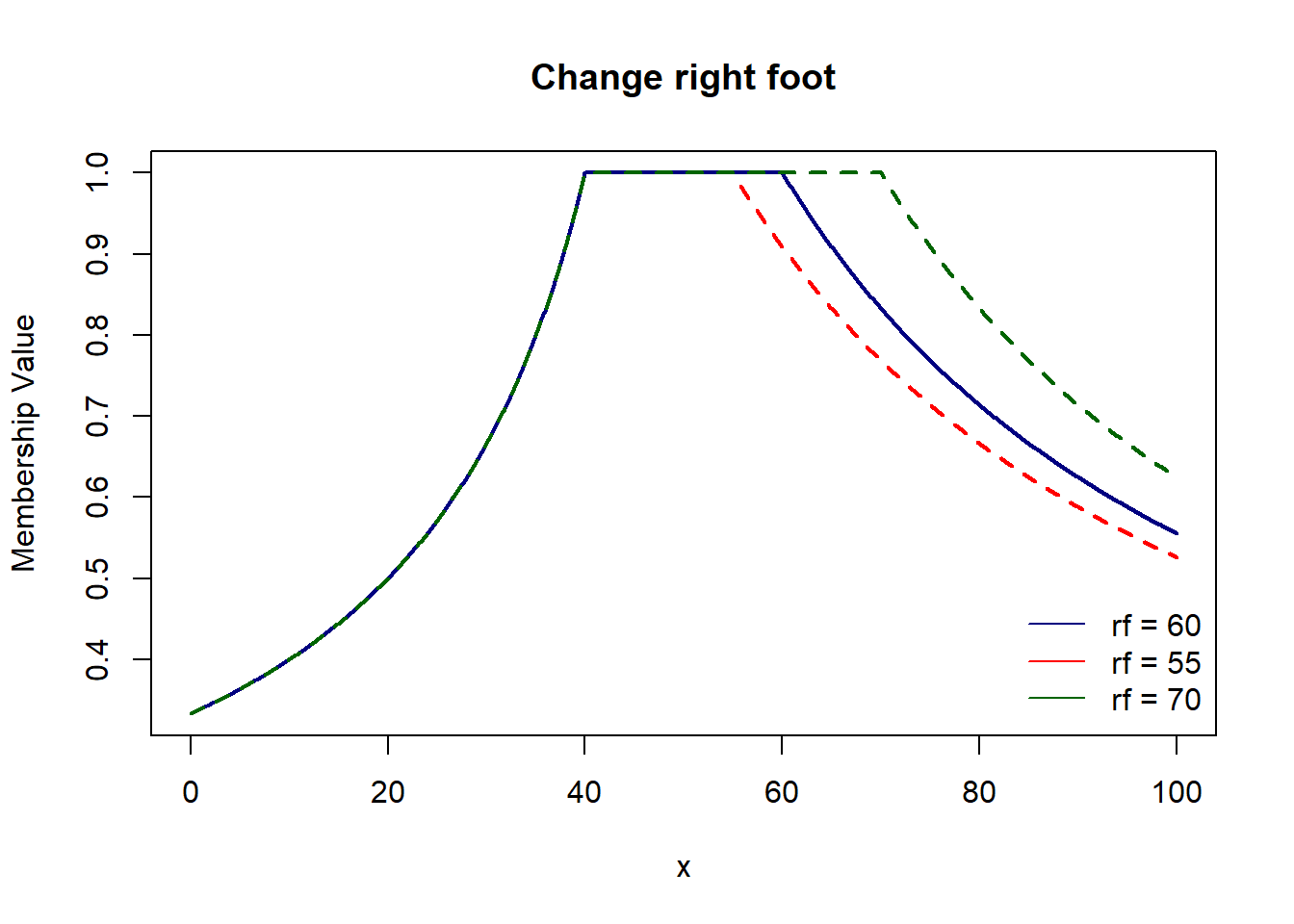
4 Parameter Pi-Shaped

Here, we have 4 parameters which control respective parts of the graph : left foot & shoulder and right foot & shoulder.

Code

# pi-shaped_4 = lf/(ls+lf-x) for x < ls
#             = 1            for ls <= x <= rs
#             = rf/(x-rs+rf) for x >= rs

pi_shaped4 = function(x, lf, ls, rf, rs){
  ifelse(x <= ls, lf/(ls+lf-x), ifelse(x <= rs, 1, rf/(x-rs+rf)))
}
plot(domain, pi_shaped4(domain, 20, 40, 50, 60), col='navy', lwd=2, type='l',
     xlab='x', ylab='Membership Value', main='Pi-Shaped Membership Function')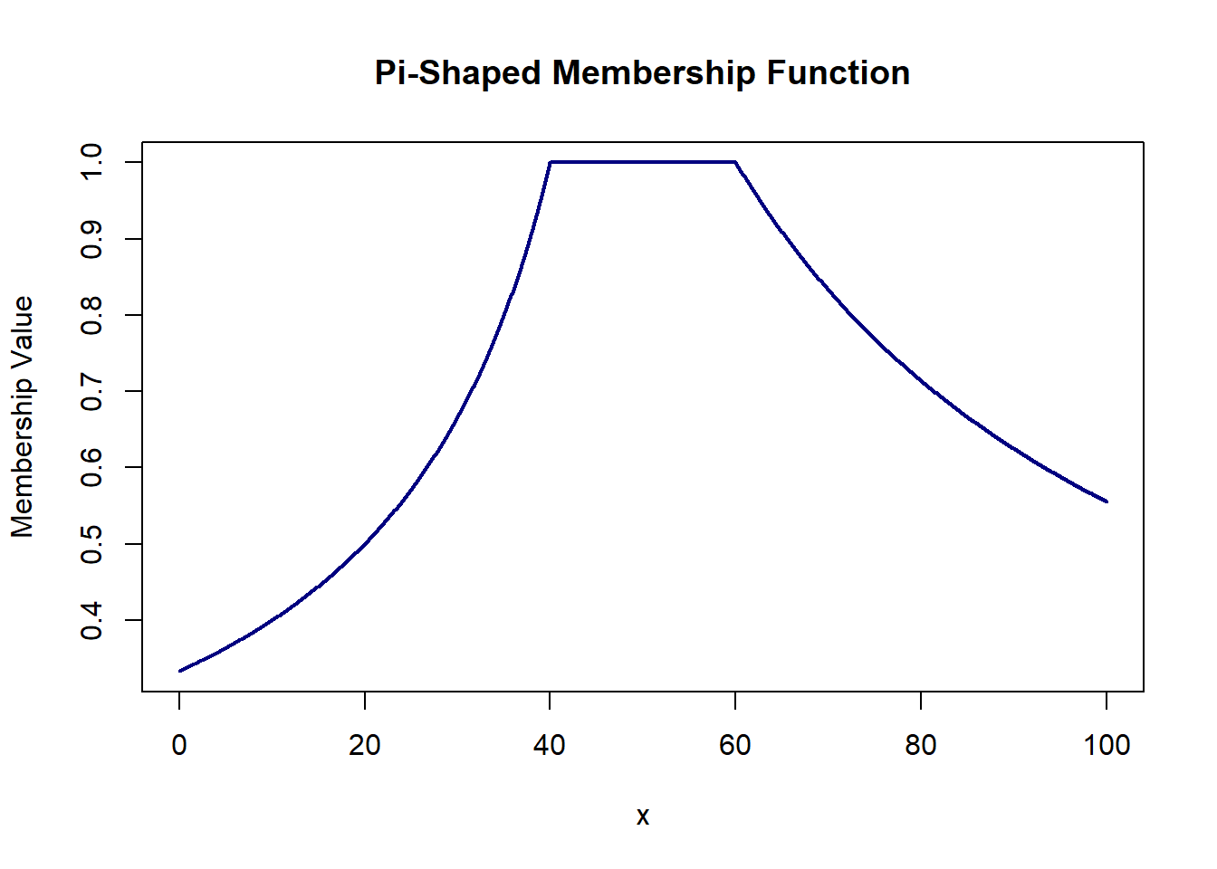

Changing Parameters

Code

# s-shaped = 0                     for x <= a
#          = 2*((x-a)/(b-a))^2     for a <= x <= (a+b)/2
#          = 1 - 2*((x-b)/(b-a))^2 for (a+b)/2 <= x <= b 
#          = 1                     for x >= b

s_shaped = function(x, a, b){
  ifelse(x<=a, 0, ifelse(x<= (a+b)/2, 2*((x-a)/(b-a))^2,
                         ifelse(x <= b, 1 - 2*((x-b)/(b-a))^2, 1)))
}
plot(domain, s_shaped(domain, 20, 50), col='navy', lwd=2, type='l',
     xlab='x', ylab='Membership Value', main='S-Shaped Membership Function')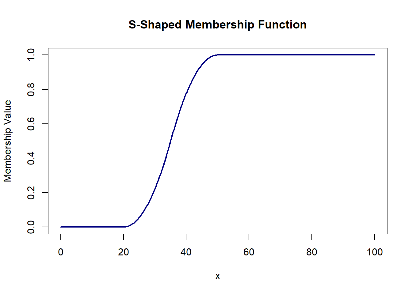

Nomenclatures

Understanding the terminology used in fuzzy logic is crucial for navigating the complexities of its concepts and applications. In the following tabs, key terms related to fuzzy sets are outlined, to serve as a foundation for our exploration of fuzzy logic.

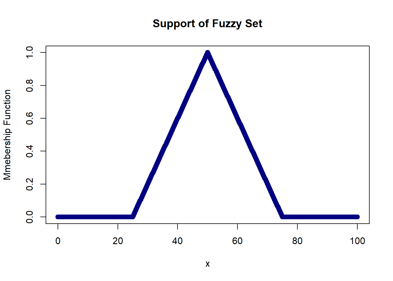
The support of a fuzzy set is defined as the crisp set of all points ‘x’ where the membership function is strictly greater than 0 (zero). Below, we have a triangular membership function. The support of this fuzzy set is represented by the set of all numbers between 25 and 75, i.e., {x : 25 < x < 75}.

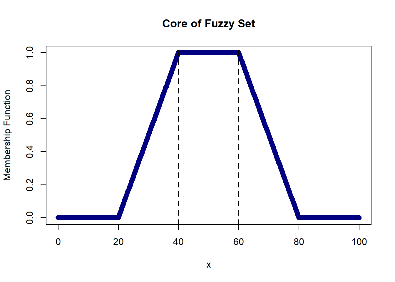
The core of a fuzzy set is defined as the crisp set of all points ‘x’ where the membership function is equal to 1. Below, we have a trapezoidal membership function where the core is defined as the set of numbers between 40 and 60, i.e., {x : 40 <= x <= 60}.

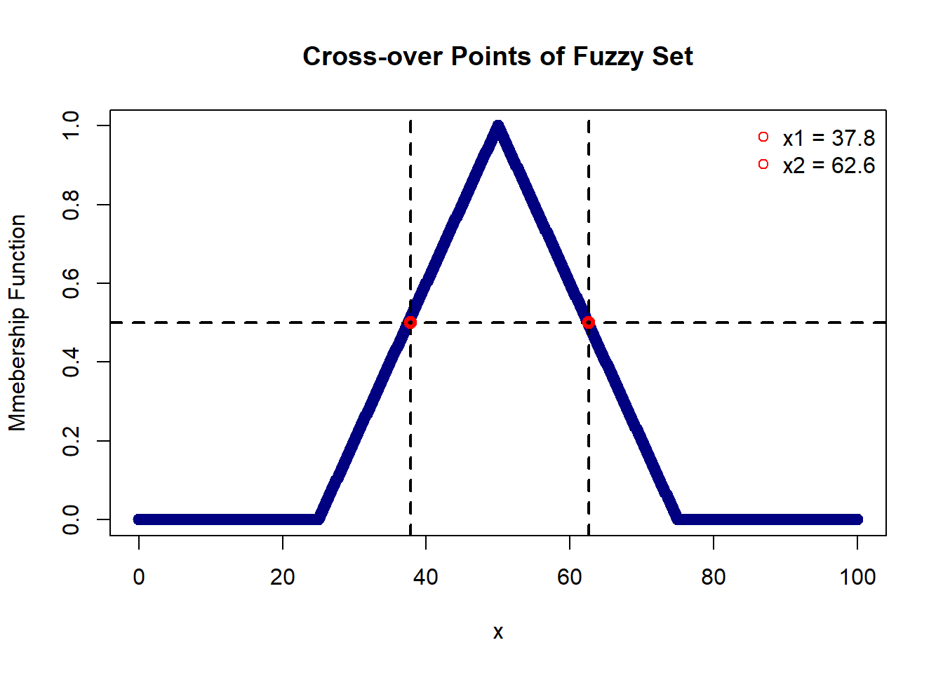
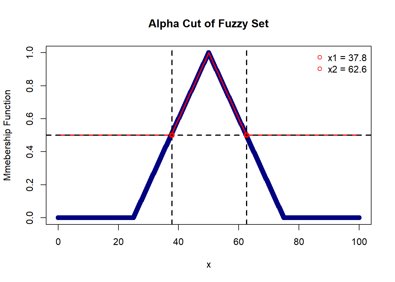
Crossover points are a crisp set of all points ‘x’ for which the membership function is equal to 0.5. Below, the crossover points are {37.8, 62.6}.

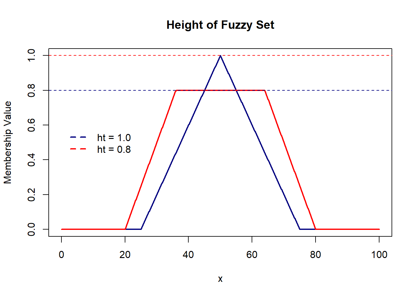
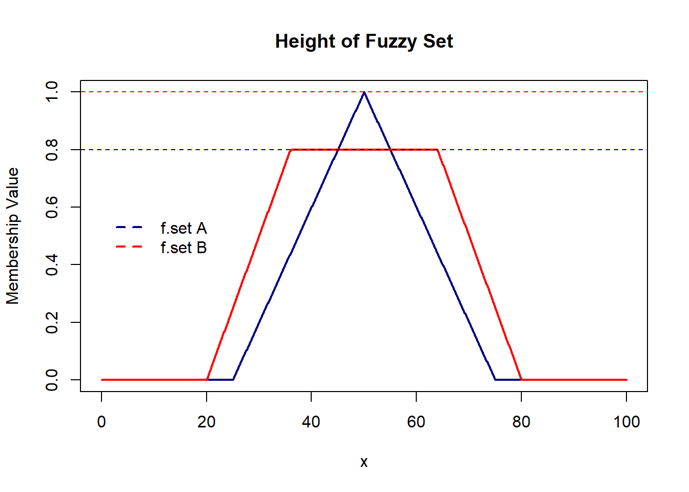
The height of a fuzzy set is the maximum membership value. Below, we have a triangular membership function with a height of 1 and a trapezoidal function with a height of 0.8.

A fuzzy set is considered ‘Normal’ if the core is non-empty or if its height is 1.
A fuzzy set is classified as ‘Sub-Normal’ if its height is less than 1.

Thus, the fuzzy set with a triangular membership function is ‘Normal’, while the one with a trapezoidal function is ‘Sub-Normal’.

It’s important to note that the height of a fuzzy set represents the degree of validity or credibility of the information expressed by the fuzzy set.

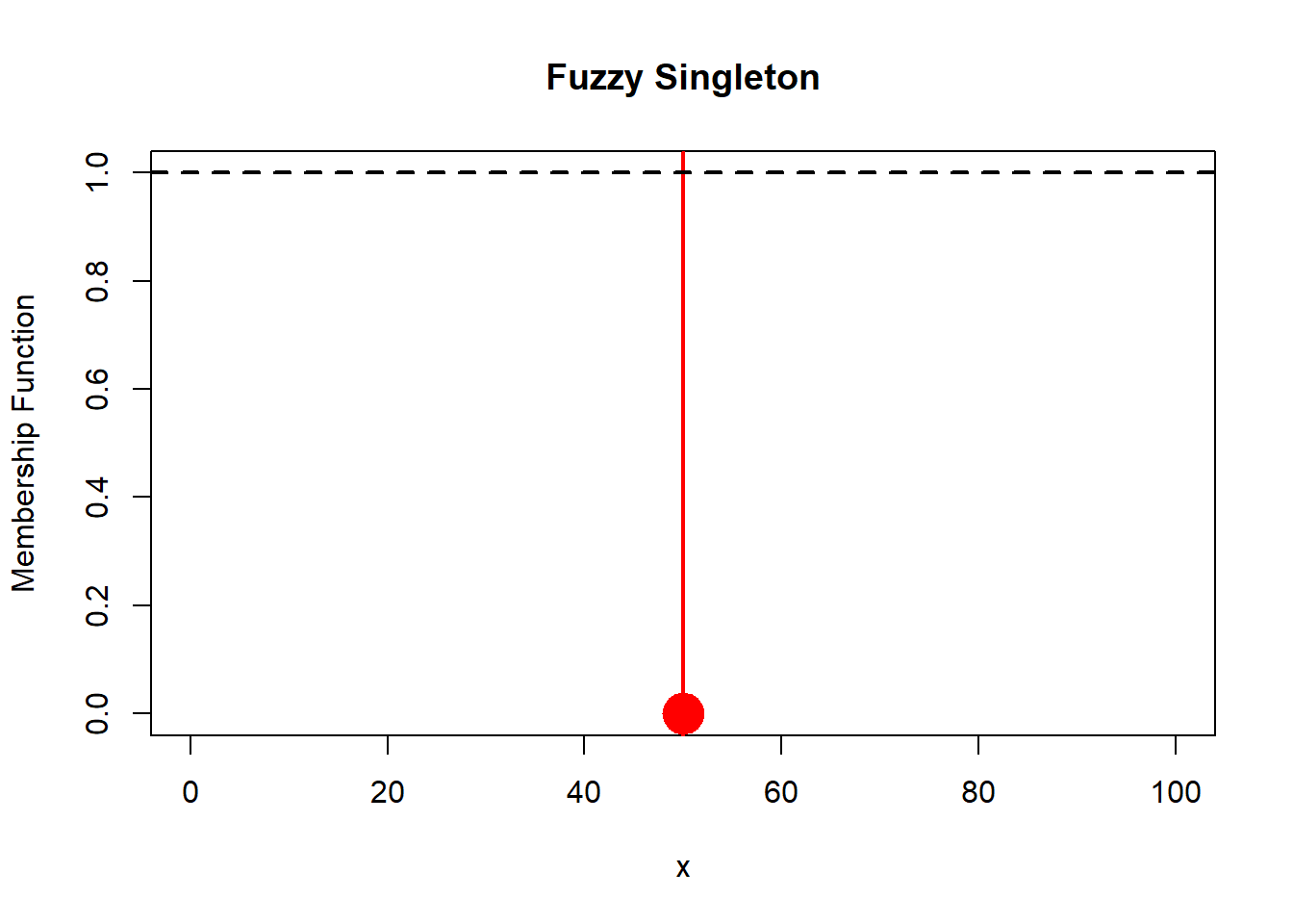
A Fuzzy Singleton occurs when the core has only one element. Alternatively, we can describe it as a fuzzy set with a support consisting of a single point with a membership value of 1. Below, the support and core of the fuzzy set are {50}.

A weak alpha-cut of a fuzzy set is a crisp set of points where the membership value is greater than or equal to alpha. A strong alpha-cut, on the other hand, is a crisp set of points where the membership value is strictly greater than alpha.

Below, we consider an alpha-cut at 0.5, resulting in a set {x : 37.8 <= x <= 62.6}, and a strong alpha-cut is represented by {x : 37.8 < x < 62.6}.

A fuzzy set A is considered convex if the following relationship holds:

$\mu_A[\lambda x_1 + (1-\lambda)x_2] >= min(\mu_A(x_1),\mu_A(x_2))$ where $\lambda \in [0,1]$

It’s important to note that the membership function exhibits a strictly monotonically increasing or decreasing, or strictly monotonically increasing-then-decreasing behavior.

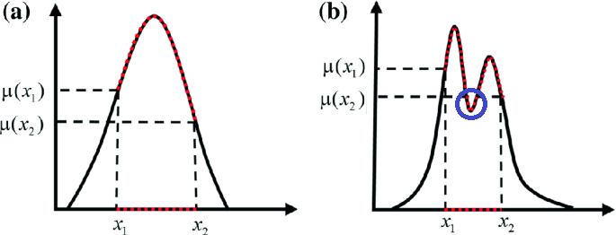
Here, in graph (a) we have a convex fuzzy set because for any two points x1 and x2, we have a portion of the graph between x1 and x2 which higher membership values than these points. Whereas in case of graph (b) we can see a dip in membership values (as circled).

A fuzzy set is classified as a fuzzy number if and only if it is both normal and convex. In the context below, Fuzzy Set A is identified as both normal and convex, thus earning the designation of a fuzzy number. However, Fuzzy Set B does not meet these criteria as it is sub-normal, therefore it is not considered a fuzzy number

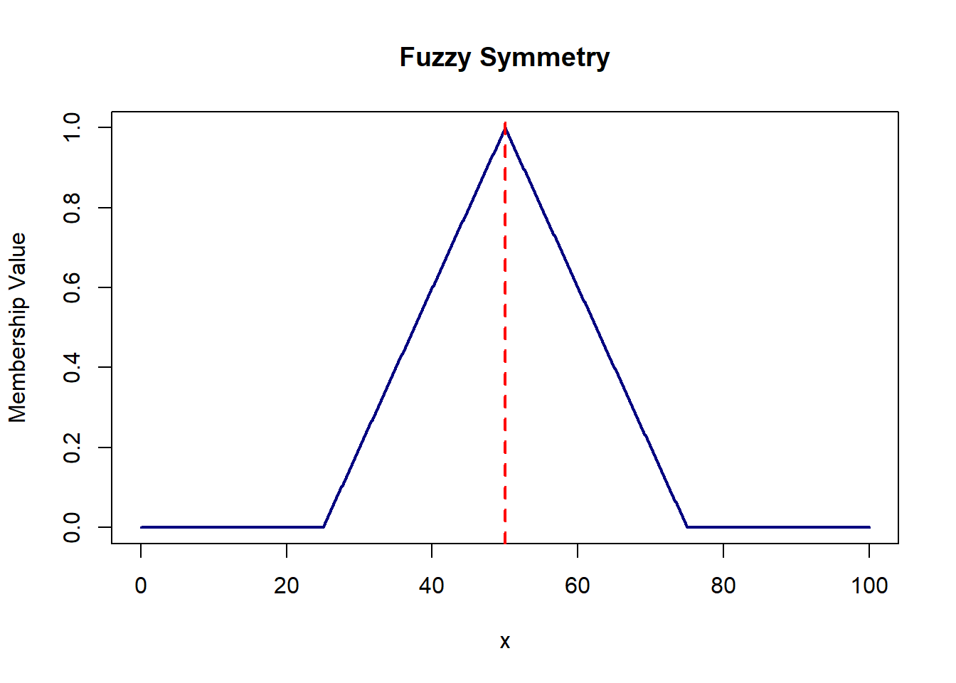
Fuzzy Set A is symmetric if $\mu_A(x)$ is symmetric around a certain point ‘c’ i.e. $\mu_A(c+x) = \mu_A(c-x);\forall x \in X$. In the example below, the membership values to the left and right of x=50 are equal, indicating symmetry in the fuzzy set.

Bandwidth is a metric exclusively defined for a fuzzy number, representing the distance between two unique crossover points. Referring to the example discussed under the crossover points section with alpha = 0.5 and x1 = 37.8 and x2 = 62.6, the bandwidth is calculated as the absolute difference between x1 and x2, yielding:

Bandwidth = | x1 - x2 | = |62.6 - 37.8| = 24.8.

Fuzzy Set Operations

Fuzzy set operations extend classical set operations to accommodate the nuanced degrees of membership inherent in fuzzy logic. These operations enable the manipulation and combination of fuzzy sets to model complex, real-world situations with greater precision.

In the following tabs, we explore some basic fuzzy set operations and their code implementation in R.

Union of two fuzzy sets is given by a set where x either belongs to A or B with membership function $$\mu_{AUB}(x) = max[ \mu_A(x), \mu_B(x)]$$

Code

plot(domain, triangle(domain, 25, 50, 75), col='navy', 
     xlab='x', ylab='Membership Value', main='Union', 
     type='l',lwd=2)
lines(domain, triangle(domain, 10, 40, 80), col='black',lwd=2)
lines(domain, pmax(triangle(domain, 25, 50, 75),
                   triangle(domain, 10, 40, 80)),lwd=5,lty=2,col='red')
legend('topright', c('A','B','A U B'),col=c('navy','black','red'), lty=1,lwd=2,bty='n')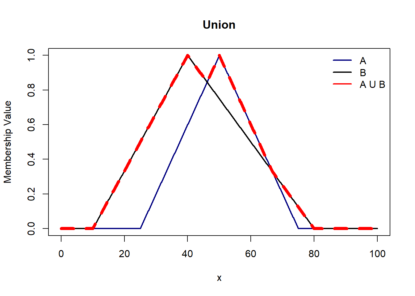

Intersection of two fuzzy sets is given by a set where x belongs to A AND B with membership functions $$\mu_{A∩B}(x) = min( \mu_A(x), \mu_B(x))$$

Code

plot(domain, triangle(domain, 25, 50, 75), col='navy', 
     xlab='x', ylab='Membership Value', main='Intersection', 
     type='l',lwd=2)
lines(domain, triangle(domain, 10, 40, 80), col='black',lwd=2)
lines(domain, pmin(triangle(domain, 25, 50, 75),
                   triangle(domain, 10, 40, 80)),lwd=5,lty=2,col='red')
legend('topright', c('A','B','A ∩ B'),col=c('navy','black','red'), lty=1,lwd=2,bty='n')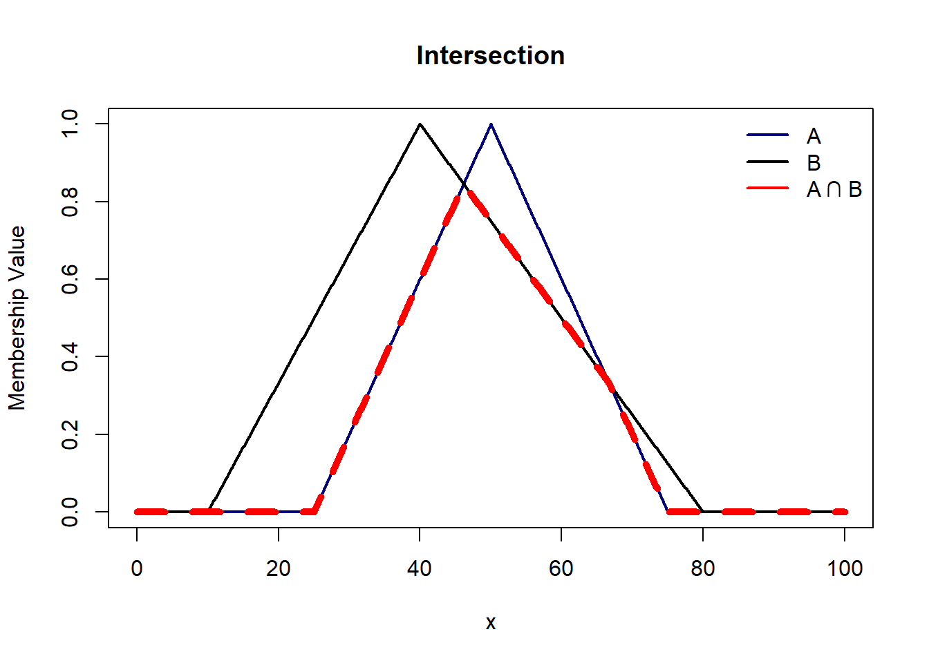

Two fuzzy sets A and B are equal iff $\mu_A(x) = \mu_B(x)$ $\forall x \in X$.

For e.g. A = { (1,0.1), (2, 0.7), (3, 0.8) } = B.

Fuzzy set A is subset of B iff $\mu_A(x) =< \mu_B(x)$ $\forall x \in X$.

For e.g. A = { (1,0.1), (2, 0.7), (3, 0.8) } and B = { (1,0.2), (2, 0.75), (3, 0.89) }. Clearly A is subset of B.

Complement of Fuzzy set A is given by A’ = {x | x not in A} with membership function given by $\mu_A'(x) = 1- \mu_x(A)$ $\forall x \in X$.

Code

plot(domain, triangle(domain, 25, 50, 75), col='navy', 
     xlab='x', ylab='Membership Value', main='Complement', 
     type='l',lwd=2)
lines(domain, 1-triangle(domain, 25, 50, 75), col='red',lwd=2)
legend(x=0,y=0.6, c('A','A complement'),col=c('navy','red'), lty=1,lwd=2,bty='n')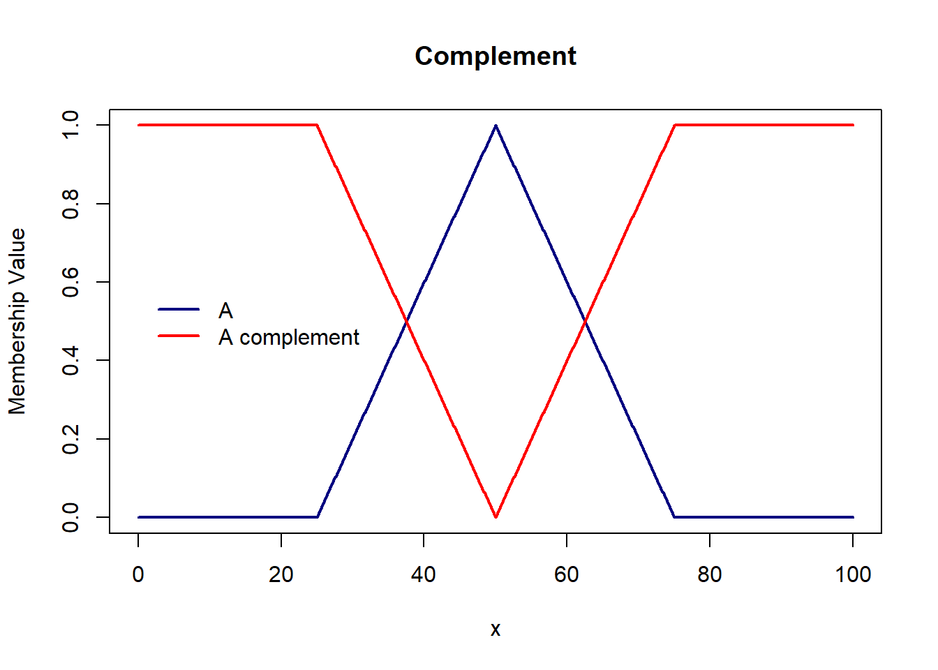

There are 3 ways we can take complements with regards to fuzzy sets. We saw the basic complement above, there are two more classes called Sugeno’s class and Yager’s class of complement.

Sugeno’s class of complement is defined as $c_\lambda(\mu_A(x)) = {1-\mu_A(x)} / {1 + \lambda \mu_A(x)}$ where $\lambda \in (-1, \infty)$. For $\lambda = 0$ we go back to basic complement.

Take an example of a discrete fuzzy set A = { (1, 0.7),(2, 0.5),(3, 0.1),(4, 0.6) } and $\lambda$ = {-0.8,0,1,2}.

Code

x = c(1,2,3,4)
m = c(0.7,0.6,0.5,0.1)
lambda = c(-0.8,0,1,2)

c_0.8 = (1-m)/(1+lambda[1]*m) # for lambda = -0.8
c_0 = (1-m)/(1+lambda[2]*m)   # for lambda = 0
c_1 = (1-m)/(1+lambda[3]*m)   # for lambda = 1
c_2 = (1-m)/(1+lambda[4]*m)   # for lambda = 2

sugeno = round(rbind(c_0.8, c_0, c_1, c_2),3)
sugeno

       [,1]  [,2]  [,3]  [,4]
c_0.8 0.682 0.769 0.833 0.978
c_0   0.300 0.400 0.500 0.900
c_1   0.176 0.250 0.333 0.818
c_2   0.125 0.182 0.250 0.750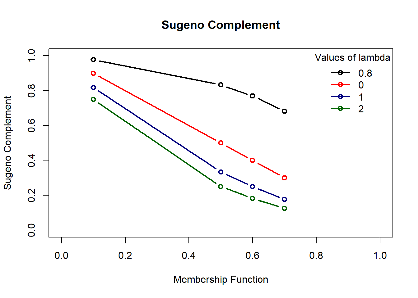

Yager’s class of complement is defined as $c_w(\mu_A(x)) = [1-\mu_A(x)^w]^{1/w}$ where $w \in (0, \infty)$. For $\lambda = 0$ we go back to basic complement.

Take an example of a discrete fuzzy set A = { (1, 0.7),(2, 0.5),(3, 0.1),(4, 0.6) } and $\lambda$ = {-0.8,0,1,2}.

Code

x = c(1,2,3,4)
m = c(0.7,0.6,0.5,0.1)
w = c(0.5,1,2,3)

w_0.5 = (1-m^w[1])^(1/w[1]) # for w = 0.5
w_1 = (1-m^w[2])^(1/w[2])   # for w = 1
w_2 = (1-m^w[3])^(1/w[3])   # for w = 2
w_3 = (1-m^w[4])^(1/w[4])   # for w = 3

yager = round(rbind(w_0.5, w_1, w_2, w_3),3)
yager

       [,1]  [,2]  [,3]  [,4]
w_0.5 0.027 0.051 0.086 0.468
w_1   0.300 0.400 0.500 0.900
w_2   0.714 0.800 0.866 0.995
w_3   0.869 0.922 0.956 1.000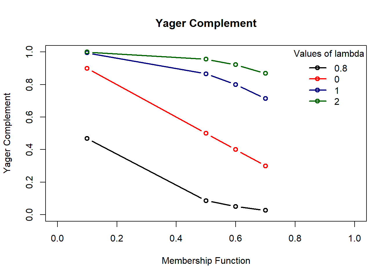

A complement ‘c’ is a function which converts a fuzzy set A, to another set $A^c$. The function ‘c’ must satisfy the following axioms:

Boundary Condition i.e. c(0) = 1 and c(1) = 0
Monotonic non-increasing
Continuity
Involution

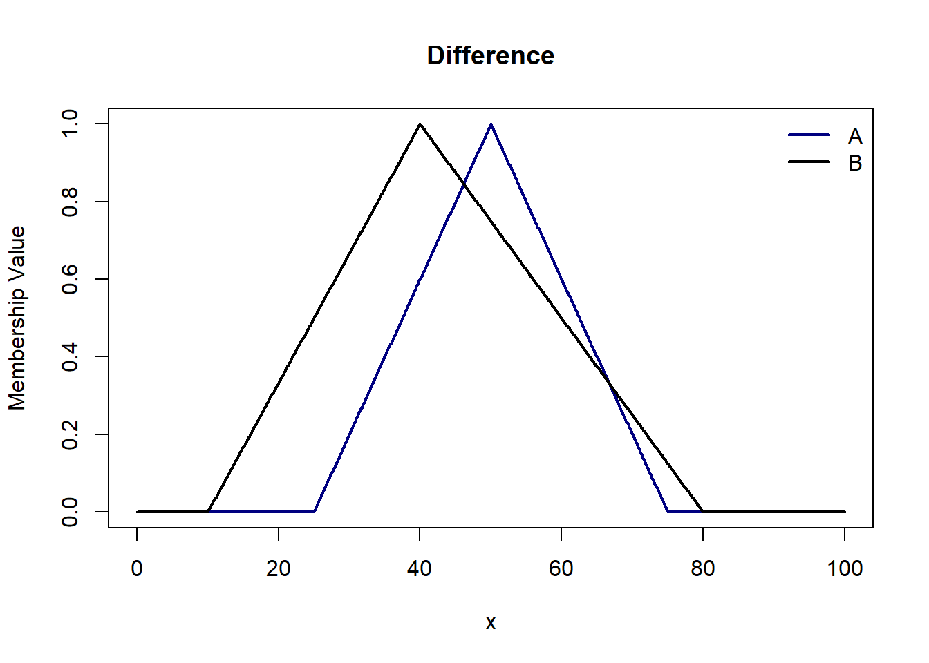
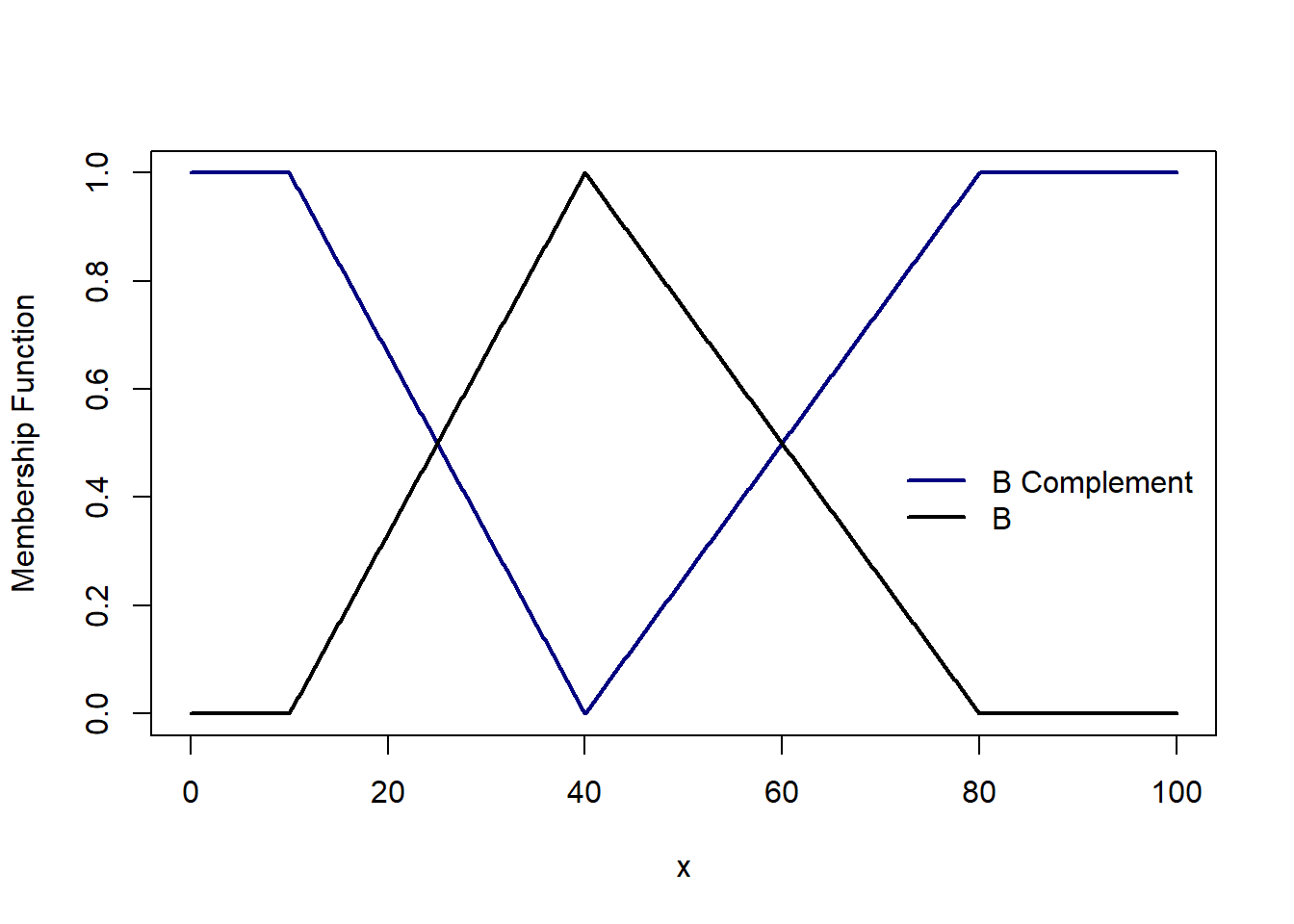
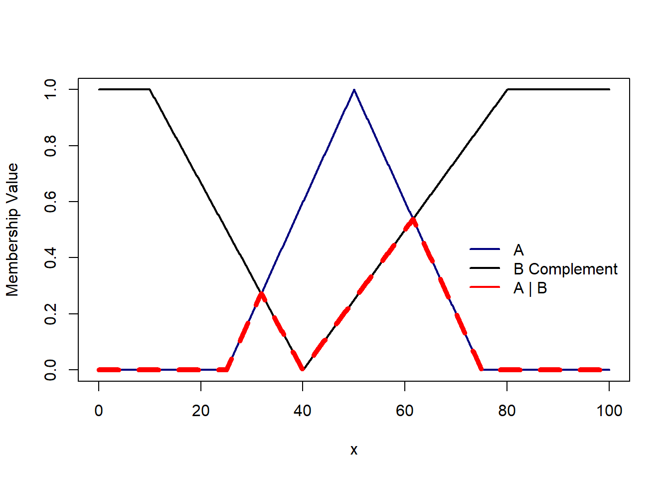
A - B i.e. A | B is a set where x belong to A and does not belong to B i.e. the union of A and B complement. The membership function is $$\mu_{A|B}(x) = min( \mu_A(x), 1-\mu_B(x))$$

T- & S-Norm Operators

T-norm and S-norm operations are pivotal in fuzzy logic, enabling the precise handling of intersections and unions within fuzzy sets. These operations form the mathematical backbone for modeling “and” and “or” conditions, respectively, facilitating nuanced decision-making in environments characterized by uncertainty and ambiguity.

In the following tabs, we see different types of T- and S-Norm Operators and their implementation in R.

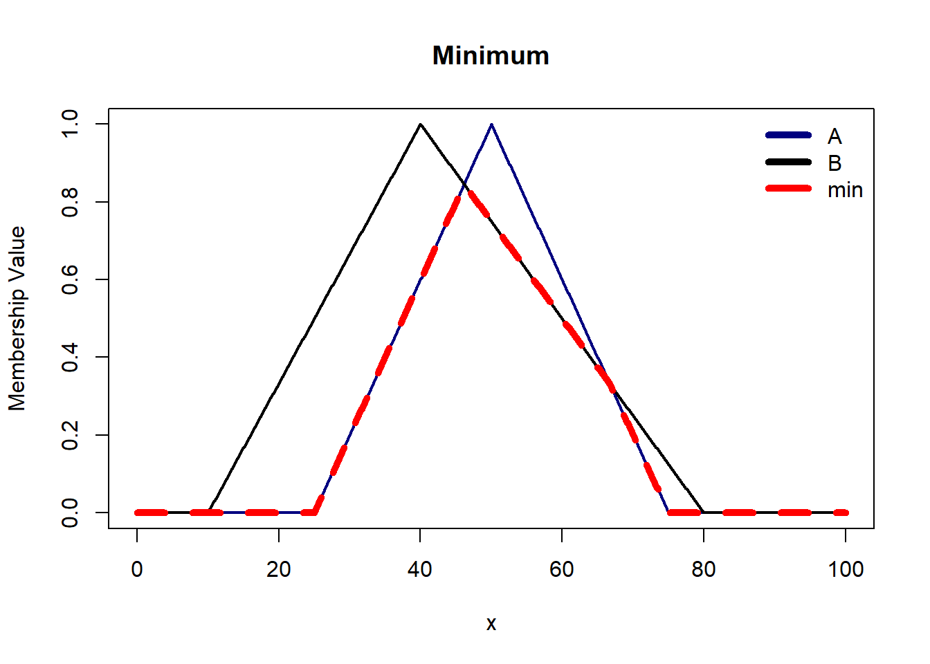
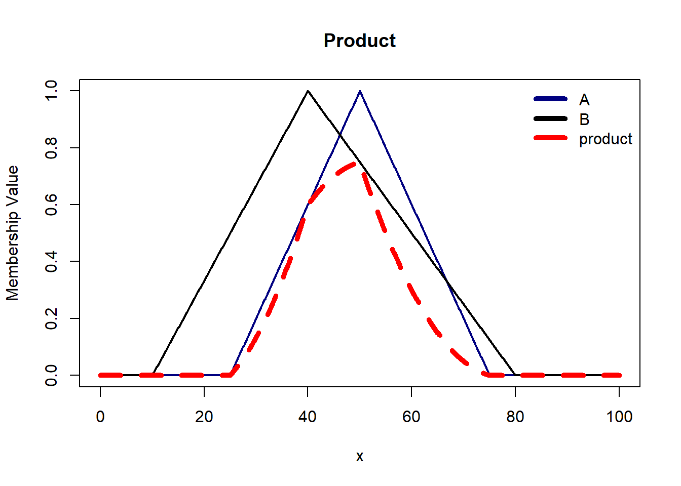
T Norm Operators are mapping functions that transform the membership functions of fuzzy sets A and B into a single truth value.

Minimum $T_{min} = min(\mu_A(x), \mu_B(x))$
Algebraic Product $T_{product} = \mu_A(x) * \mu_B(x)$
Bounded Product $T_{bp} = min(0, \mu_A(x) + \mu_B(x)-1)$
Drastic Product $T_{dp} = \mu_A(x)$ for $\mu_B(x) = 1$; $\mu_B(x)$ for $\mu_A(x) = 1$; 0 elsewhere

Suitability

Minimum is the most commonly used t-norm operator. It ensures that the truth value of the conjunction is not greater than truth value of the individual proposition. It is conservative in nature.
Product is suitable when the interaction between two fuzzy propositions are naturally interpreted as multiplicative processes, thus, capturing the combined influence of both. Here we lay no emphasis on either the weaker or stronger proposition.
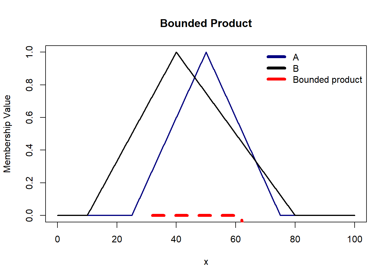
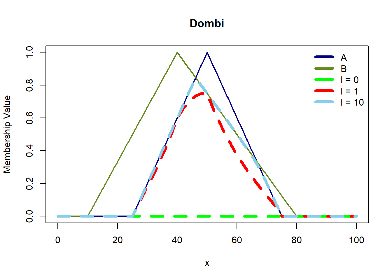
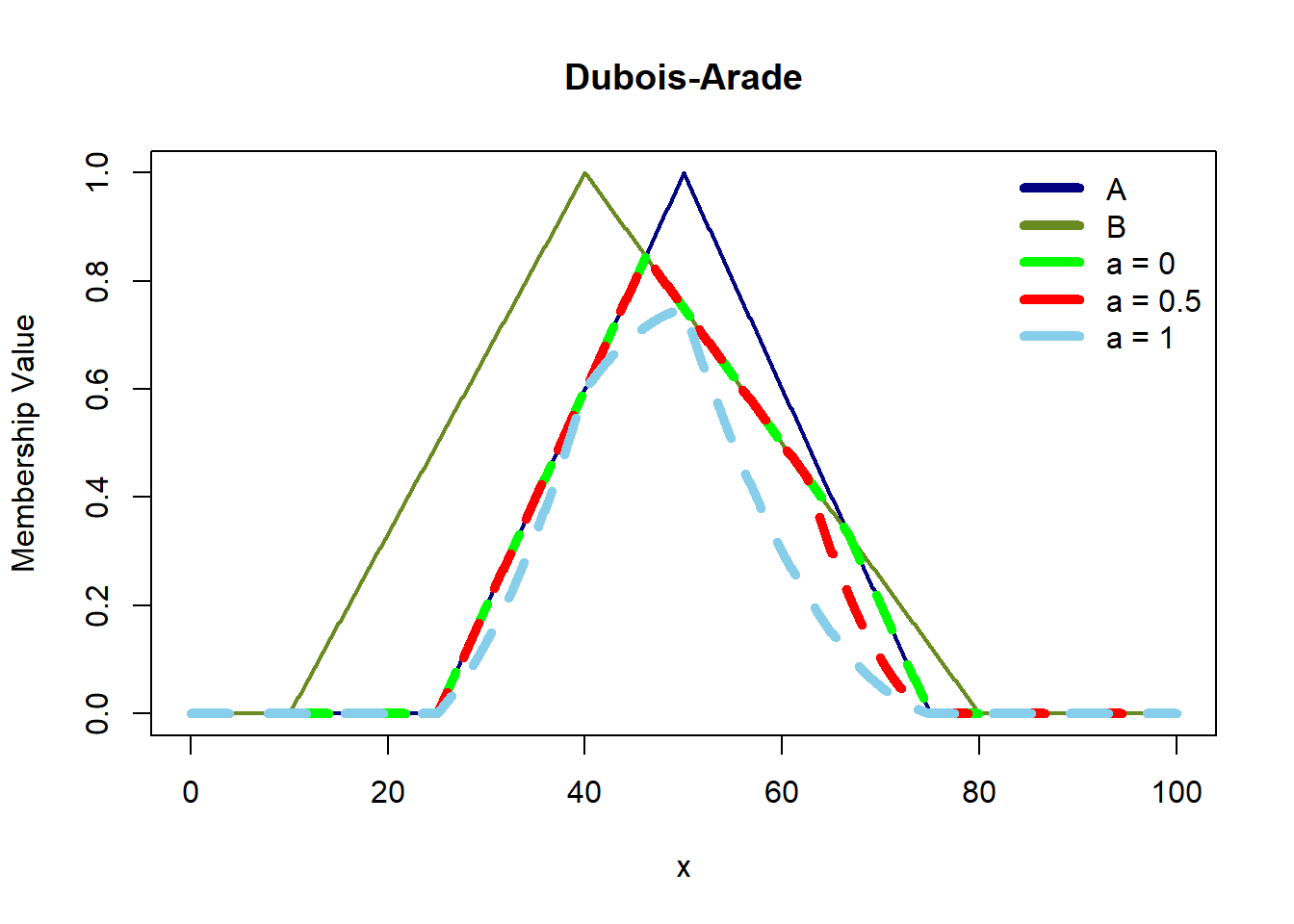
Bounded Product is suitable when you want to limit the influence of one proposition when the other is weak. It bounds the product to ensure that the conjunction does not exceed a certain threshold. In situations where there is imprecision /uncertainty in the input data, the bounded product can be a good choice as it helps mitigate the impact of extreme values and provides a more gradual transition in the truth values.
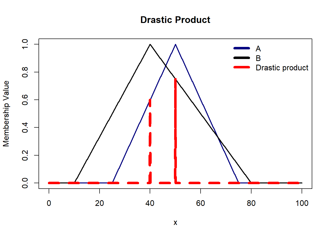
Drastic Sum is suitable when we want to emphasize the importance of the weakest proposition in the conjunction i.e. focus more on the minimum truth value.

S Norm Operators are mapping functions that transform membership functions of fuzzy sets A and B into an unified output.

Maximum $S_{max} = max(\mu_A(x), \mu_B(x))$
Probabilistic Sum $S_{sum} = \mu_A(x) + \mu_B(x) - \mu_A(x) * \mu_B(x)$
Bounded Sum $S_{bs} = max(1, \mu_A(x) + \mu_B(x))$
Drastic Sum $S_{ds} = \mu_A(x)$ for $\mu_B(x) = 0$; $\mu_B(x)$ for $\mu_A(x) = 0$; 1 elsewhere

Suitability

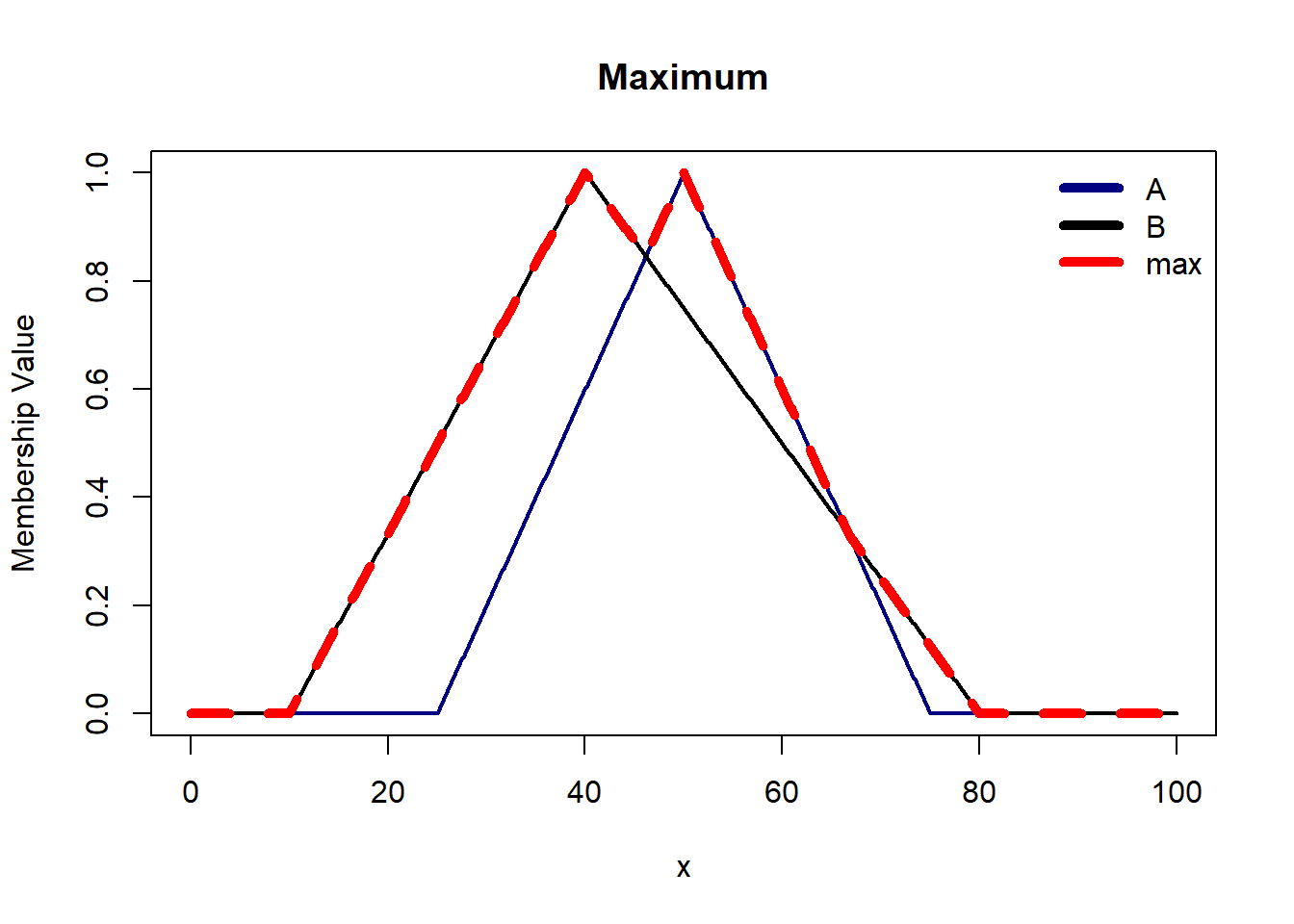
Maximum is the most commonly used s-norm operator. Like minimum t-norm, max s-norm is also conservative in nature. It ensures that the truth value of the disjunction is not less than the maximum truth value of the individual propositions.
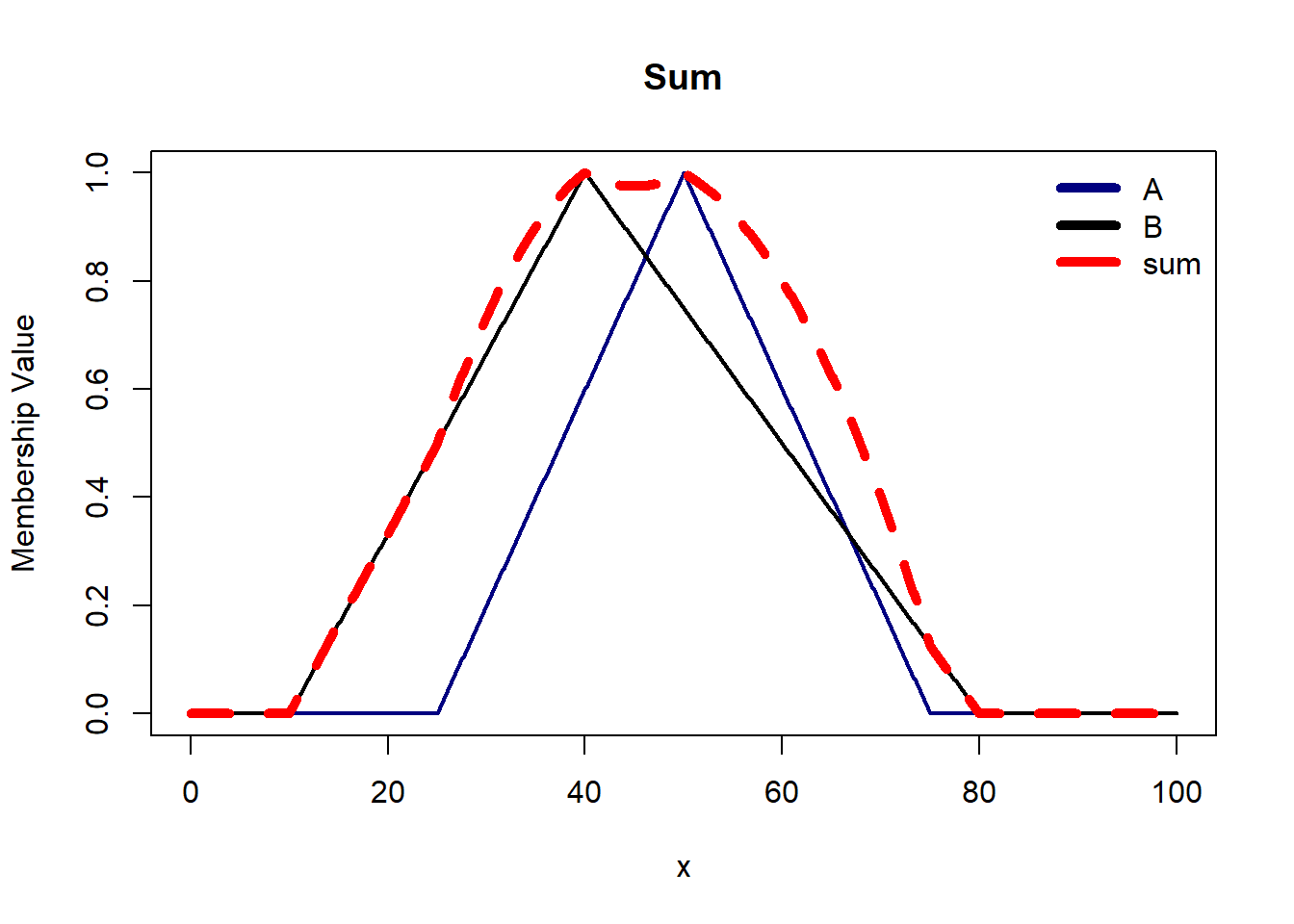
Algebraic Sum provides a smooth transition between the disjunction of two propositions and their conjunctions. The $ab$ term captures the interaction/overlap between the two propositions. Subtracting $ab$ ensures that the commonality between propositions is not counted twice.
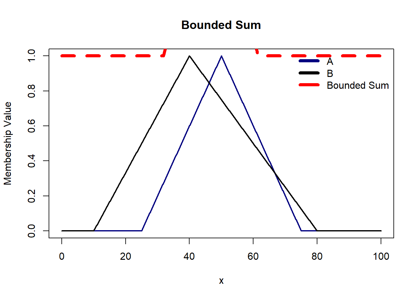
Bounded Sum limits provides controlled aggregation of fuzzy propositions as we limit the output to a maximum of 1. Thus, it prevents the output from being overly influenced by extreme values, contributing to a more stable and robust fuzzy logic system.
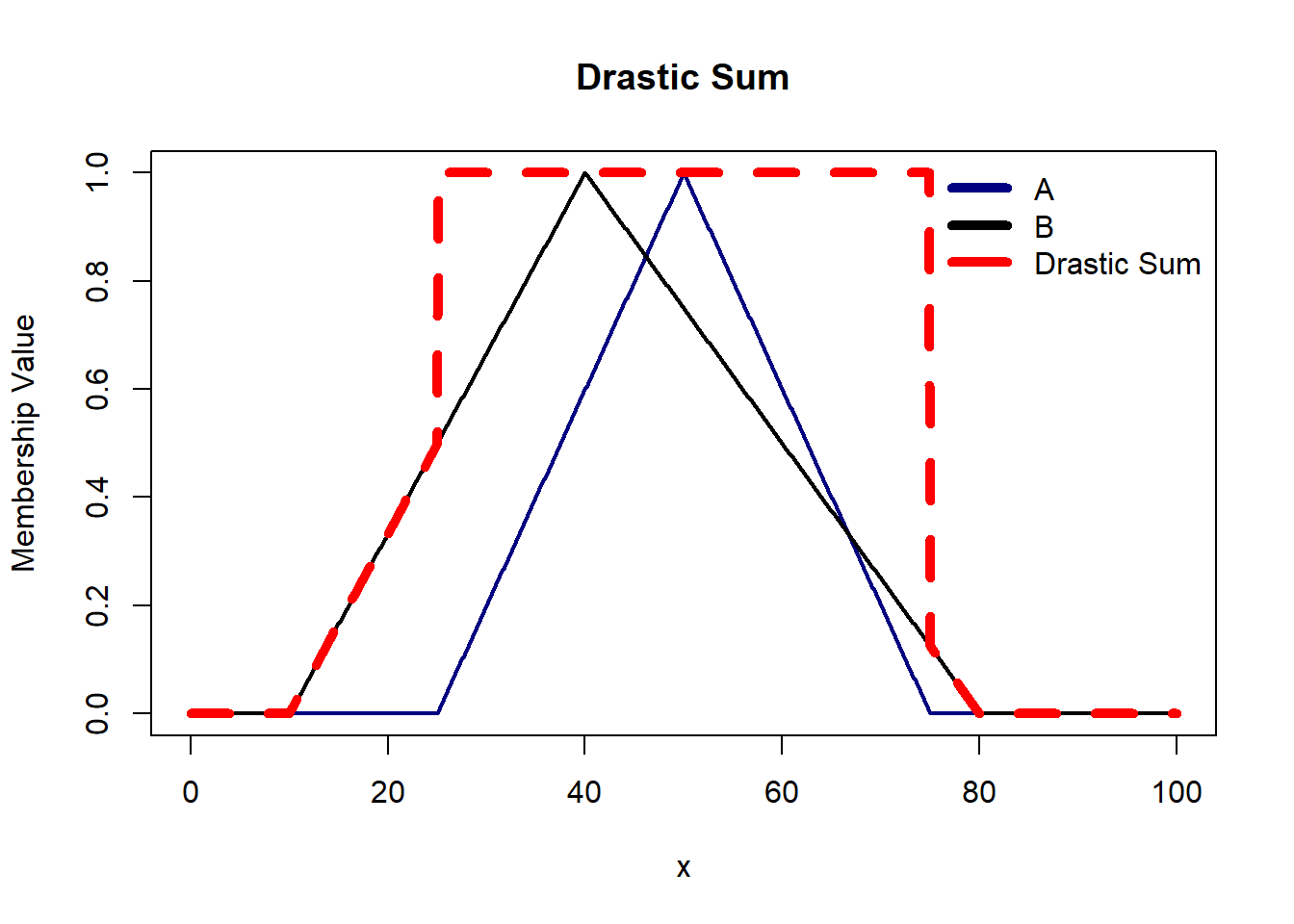
Drastic Sum tends to avoid middle-ground truth values. It emphasizes a clear-cut decision by assigning a truth value of 1 when at least one proposition is true. This is useful when we don’t want ambiguity in our output.

There are some axioms t-norm and s-norm operators must satisfy:

Boundary Condition
- For t-norms, t(a,1) = a.
- For s-norms, s(a,0) = a.
Monotonicity

If b <= c, then o(a,b) <= o(a, c). This holds true for both t-norm and s-norm. Here, ‘o’ represents t- and s-norms.
Commutative

o(a, b) = o(b, a).
Associative

o(a, o(b,c)) = o( o(a,b), c).
Continuity
Idempotency

o(a, a) = a.

DOMBI

$T_{dombi} = 1/[{1 + [(1/\mu_A(x)-1)^\lambda + (1/\mu_B(x)-1)^\lambda]^{1/\lambda}}]$ where, $\lambda \in [0,\infty)$

DUBOIS ARADE’S

$T_{dubois-arade} = \mu_A(x)*\mu_B(x)/max(\alpha,\mu_A(x),\mu_B(x))$ where, $\alpha \in [0,1]$

YAGER

$T_{yager} = 1 - min(1, ((1-\mu_A(x))^w+((1-\mu_B(x))^w)^{1/w})$ where, $w \in (0,\infty)$

DOMBI

$S_{dombi} = 1/[{1 + [(1/\mu_A(x)-1)^{-\lambda} + (1/\mu_B(x)-1)^{-\lambda}]^{-1/\lambda}}]$ where, $\lambda \in [0,\infty)$

DUBOIS ARADE’S

$S_{dubois-arade} = numerator/denominator$
numerator = $\mu_A(x)+\mu_B(x)-\mu_A(x)*\mu_B(x) - min(1-\alpha,\mu_A(x),\mu_B(x))$
denominator = $max(\alpha,1-\mu_A(x),1-\mu_B(x))$
where, $\alpha \in$ [0,1]

YAGER

$S_{yager} = min(1, (\mu_A(x)^w+\mu_B(x)^w)^{1/w})$ where, $w \in (0,\infty)$

Fuzzy Relation

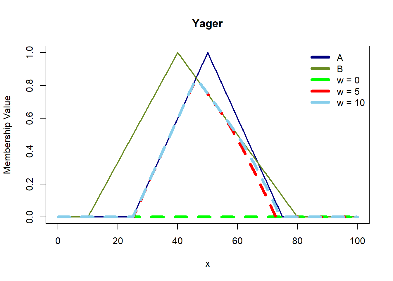
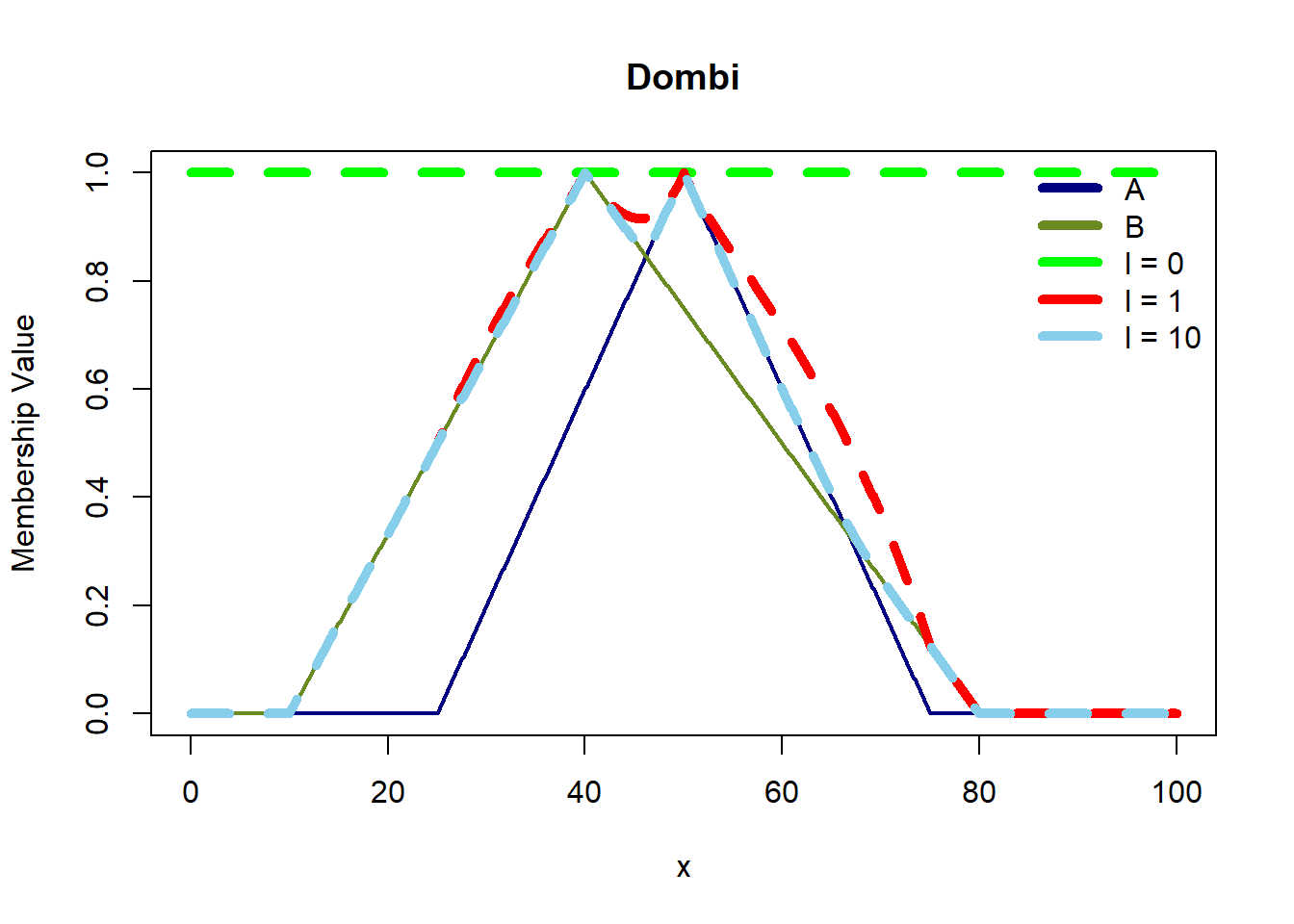
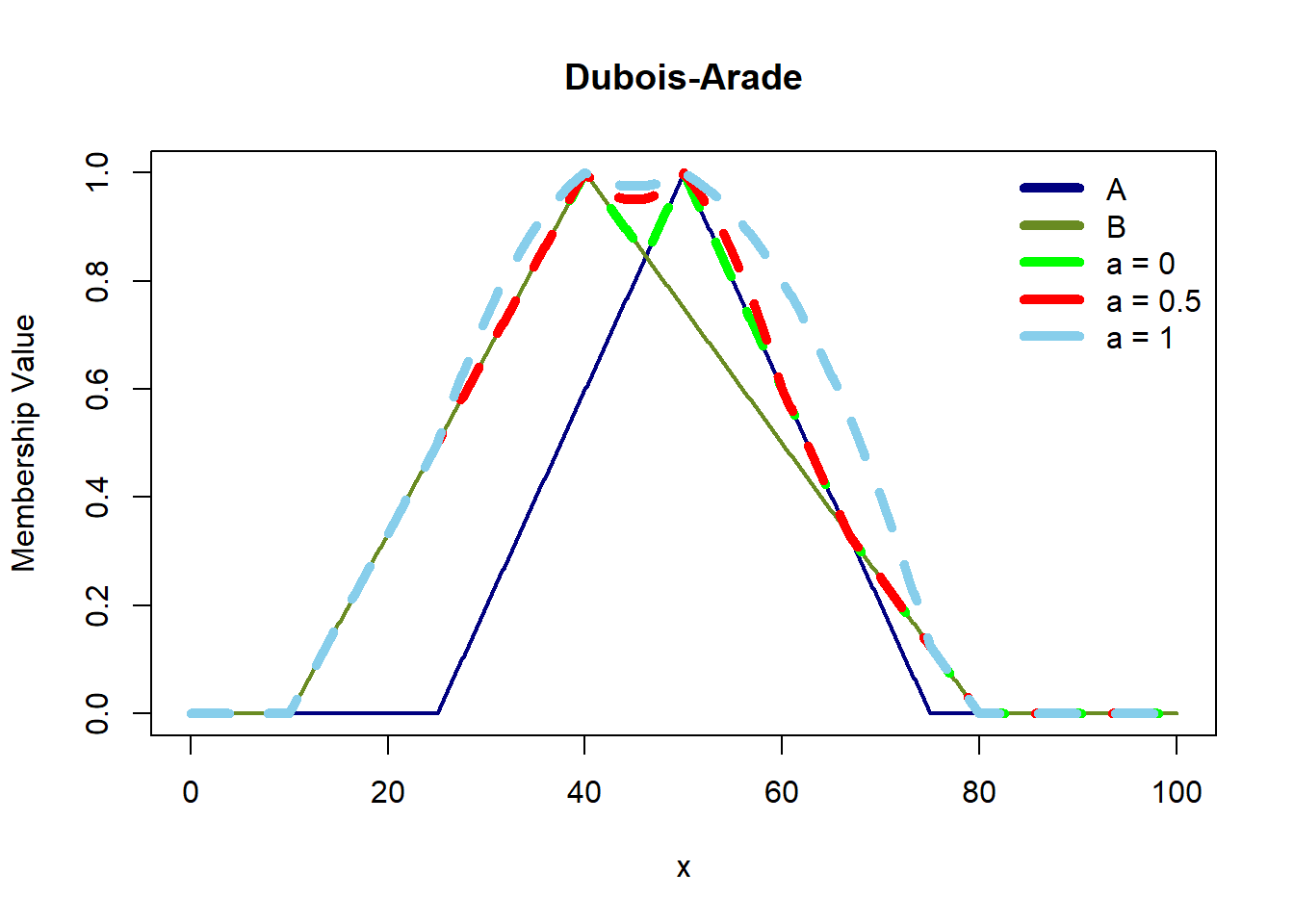
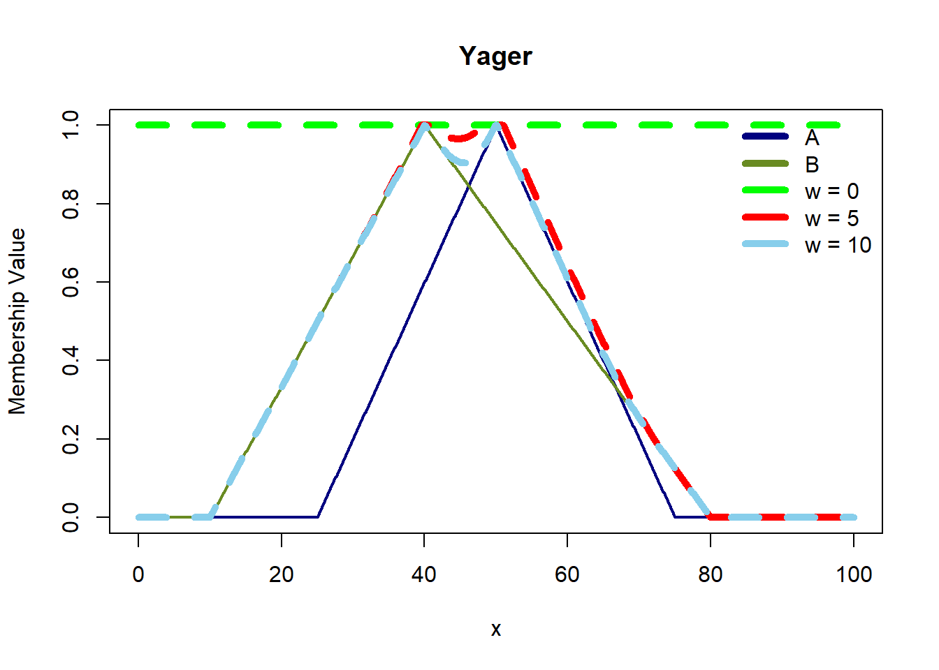
In fuzzy logic, relations extend beyond crisp sets to encompass fuzzy sets, allowing for a more nuanced interpretation of how elements relate to each other. For crisp sets A and B, a relation (R) is a subset of the Cartesian product (A x B), consisting of ordered pairs ((x, y)) where (x $\in$ A) and (y $\in$ B). In contrast, for fuzzy sets A and B, a fuzzy relation (R) on (A x B) is defined by ordered pairs $(((x, y), \mu{A \times B}(x,y)))$, where each pair is associated with a membership degree $(\mu{A \times B}(x,y))$ determined by the minimum of the membership values of x $\in$ A and (y $\in$ B, denoted as $(\min(\mu_A(x), \mu_B(y)))$.

Consider fuzzy sets A and B, with memberships as follows:

A = 0.2/$x_1$ + 0.5/$x_2$ + 1/$x_3$
B = 0.3/$y_1$ + 0.9/$y_2$

The fuzzy relation (A B) is represented by:

A X B = { (($x_1$,$y_1$),0.2), (($x_1$,$y_2$),0.2), (($x_2$,$y_1$),0.3), (($x_2$,$y_2$),0.5), (($x_3$,$y_1$),0.3), (($x_3$,$y_2$),0.9) }

This example illustrates how each pair in the Cartesian product of A and B is assigned a membership degree, reflecting the strength of their relationship in the context of the fuzzy sets.

Similar to operations on fuzzy sets, we can apply operations of union, intersection, complement, and subset determination to fuzzy relations, allowing for flexible manipulation and analysis of relationships between fuzzy sets. This adaptability enables fuzzy logic to model complex systems where relationships and associations are not strictly binary, capturing the subtleties of real-world interactions.

For a fuzzy relation R $\subset$ AXB, the projection of R onto A and B is denoted by $R_A$ and $R_B$ respectively, with membership functions $\mu_{R_A}(x) = max_{y} \mu_R(x,y)$ and $\mu_{R_B}(x) = max_{x} \mu_R(x,y)$. In simpler terms, when dealing with the projection over x, we consider the maximum membership values over y, and vice versa.

Fuzzy relations, being multi-dimensional and defined on multiple universes of discourse, can have their dimensionality reduced through projections.

The Extension Principle serves as a foundational mechanism in fuzzy logic, facilitating the mapping of a fuzzy set across different universes of discourse. This principle not only broadens the applicability of fuzzy sets but also enables the creation of nuanced connectives that align more closely with the complexities of logical expressions. By leveraging this principle, distinctions among concepts like ‘unknown,’ ‘undefined,’ and ‘undecidable’ can be more accurately depicted, ranging from ‘definitely false’ to ‘true-ish.’

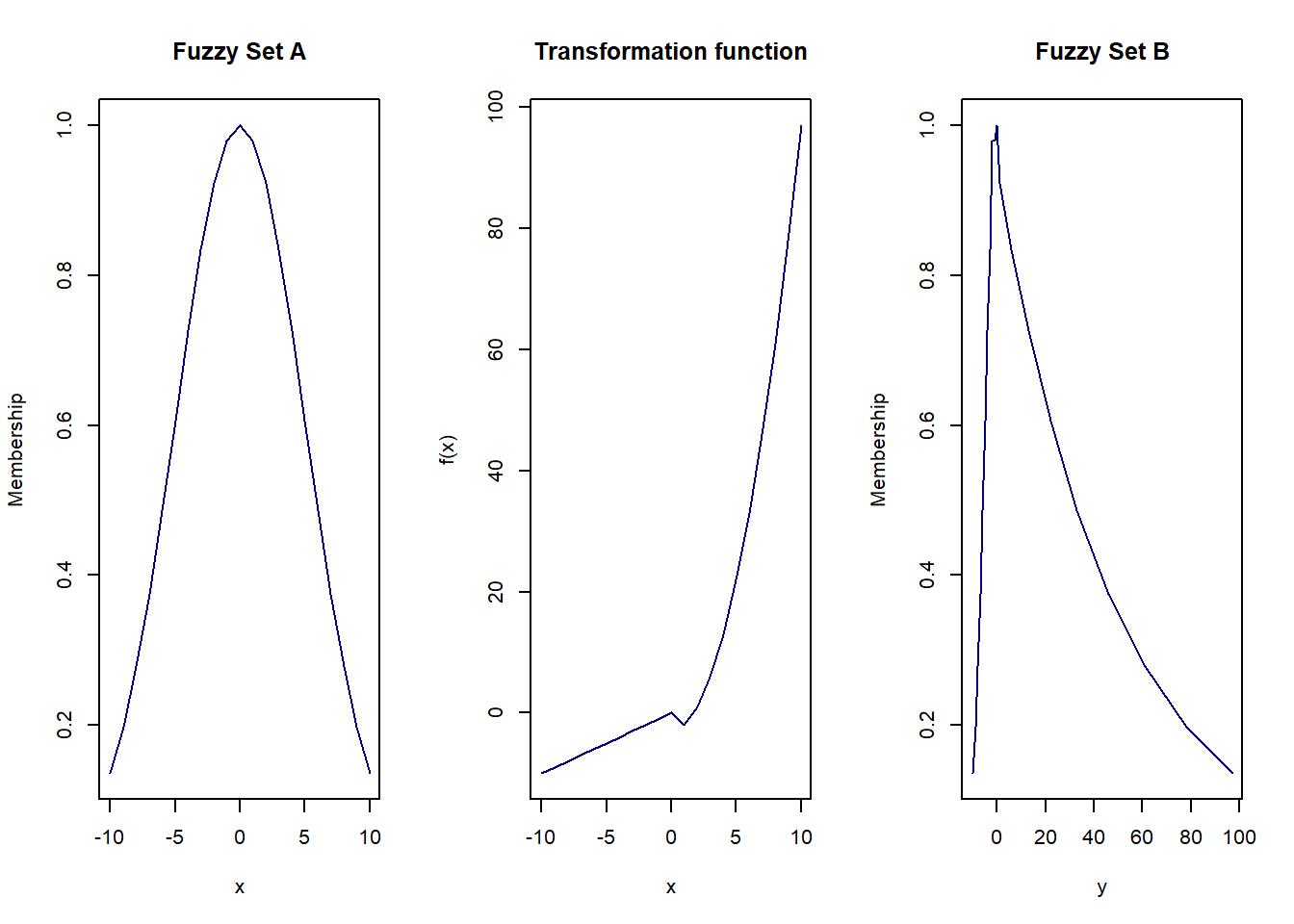
Consider a fuzzy set (A) situated within a universe of discourse (X), spanning the domain ([-10, 10]). Utilizing the Extension Principle, we can define a new fuzzy set (B) within a different universe of discourse (Y), applying the mapping function $f(x) = x^2 -3$ for (x > 0), and $f(x)=x$ otherwise. This approach allows for the transformation and reinterpretation of fuzzy set (A) in the context of (Y), demonstrating the principle’s versatility in extending fuzzy logic’s reach across varied domains.

Code

x = seq(-10,10,1) 
mux = gaussian(x, 0, 5) 

fx = function(x){ ifelse(x>0, x^2 -3, x) } 

y = fx(x)  

og_df = data.frame(x, mux, y) 
og_df

     x       mux   y
1  -10 0.1353353 -10
2   -9 0.1978987  -9
3   -8 0.2780373  -8
4   -7 0.3753111  -7
5   -6 0.4867523  -6
6   -5 0.6065307  -5
7   -4 0.7261490  -4
8   -3 0.8352702  -3
9   -2 0.9231163  -2
10  -1 0.9801987  -1
11   0 1.0000000   0
12   1 0.9801987  -2
13   2 0.9231163   1
14   3 0.8352702   6
15   4 0.7261490  13
16   5 0.6065307  22
17   6 0.4867523  33
18   7 0.3753111  46
19   8 0.2780373  61
20   9 0.1978987  78
21  10 0.1353353  97

We can see that values of y are repeating. Now, we need to arrange them and keep the maximum membership values. For e.g. for $y = -2$, $\mu_B(y) = max(0.92, 0.98) = 0.98$.

Code

library(dplyr) 
new_df = og_df %>% group_by(y) %>% summarise(max_mux = max(mux)) 
new_df

# A tibble: 20 × 2
       y max_mux
   <dbl>   <dbl>
 1   -10   0.135
 2    -9   0.198
 3    -8   0.278
 4    -7   0.375
 5    -6   0.487
 6    -5   0.607
 7    -4   0.726
 8    -3   0.835
 9    -2   0.980
10    -1   0.980
11     0   1    
12     1   0.923
13     6   0.835
14    13   0.726
15    22   0.607
16    33   0.487
17    46   0.375
18    61   0.278
19    78   0.198
20    97   0.135

Now we have our fuzzy set B sorted ! Let’s visualise them now.

Code

x = seq(-3, 3, 0.01) 
mux = gaussian(x, 0, 0.8) 
muy = gaussian(x, 0, 0.4) 
proj_df = data.frame(x = x, mux = mux, y = x, 
                     muy = muy, muxy = pmax(mux, muy))

membership <- matrix(proj_df$muxy,                       
                     nrow = length(unique(proj_df$x)),
                     ncol = length(unique(proj_df$y)))  

plot_ly(x = unique(proj_df$x), y = unique(proj_df$y), 
        z = ~membership, type = "surface") %>%     
  layout(scene = list(zaxis = list(title = "Membership Values")))

The interactive graph allows you to visualize the fuzzy relation and its projections along the x and y axes. By manipulating the graph’s orientation, you can observe the Gaussian distributions corresponding to each axis, offering a dynamic way to explore and understand the relationship between fuzzy sets.

Linguistic Hedges

Linguistic Hedges offer a refined framework for describing variables in terms that mirror natural language, encapsulating a variable’s essence through a structured quintuple: (x, T(x), X, G, M). This framework includes:

‘x’ is the name of the variable e.g. age
‘T(x)’ is term set e.g. T(x) = {young, middle-aged, old}
‘X’ is the universe of discourse e.g. X = [0,100]
‘G’ is syntactic rule which generates term in T(x) e.g.’young’ is a syntactic label
‘M’ is semantic rule which associates each linguistic value x e.g. procedure for computing membership functions

This structure allows for the nuanced expression of variables and their attributes, facilitating a more intuitive and detailed approach to categorizing and reasoning about information in fuzzy logic systems.

Primary Terms e.g. low, medium, high - these are the atomic words
Linguistic Hedges e.g. very, more or less, slight, fairly, barely, mostly, approximately - these are adverbs/adjectives.
Negation/Complement & Connectives e.g. not low, not high, low but not very low.

‘A’ is a linguistic variable characterized by a fuzzy set with membership $\mu_A(x)$. Then ‘$A^{(k)}$’ is concentration of original linguistic value expressed as :

$A^{(k)} = [\mu_A(x)]^k/x$ for k > 1

Dilation on the other hand is define for k < 1.

When concentrating, the spread or uncertainty of a fuzzy set is reduced, whereas dilation increases the spread. Concentration is particularly useful in situations where a more precise representation of a variable is required, helping to reduce uncertainty and emphasize the core elements of a fuzzy set. For example, in control systems, concentration might be employed to improve the accuracy of rule-based decisions.

On the other hand, dilation allows us to capture a broader range of possibilities, accommodating inherent variability in input data.

In the context of Explainable AI (XAI), concentration and dilation serve as tuning mechanisms to adjust the sensitivity or tolerance of a fuzzy system. These operations allow us to fine-tune the shape of membership functions, aligning the model’s behavior with our expectations. This adjustment makes the model more interpretable, contributing to a clearer understanding of its decision-making process.

Let’s take an example of a Gaussian membership function.

Code

plot(domain, gaussian(domain, 50, 10), type='l', col='navy', lwd=2, 
     xlab='x',ylab='Membership Value',main='Concentration vs. Dilation')
lines(domain, gaussian(domain, 50, 10)^2, type='l', col='red', lwd=2,lty=2)
lines(domain, gaussian(domain, 50, 10)^0.5, type='l', col='darkgreen', lwd=2,lty=2)
legend('topright',c('Original','Concentration','Dilation'), 
       col=c('navy','red','darkgreen'),lwd=2,lty=1,bty='n')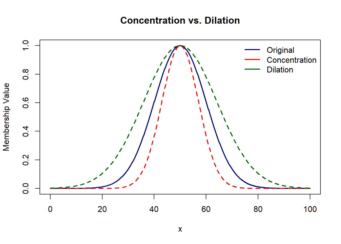

Let’s take an example and understand how to deal with composite linguistic terms. Here, we have : -

Linguistic variable x = ‘weight’
Term set T(x) = {light, heavy}
Universe of Discourse X = [-50,150]
$\mu_{light}(x) = bell(x;11,2.5,27)$ and $\mu_{heavy}(x) = bell(x;14,3.5,65)$

We have to find the fuzzy sets for these composite linguistic terms:

Light but not too Light

Let’s break this down. For “too light” we concentrate $\mu_L(x)$ with k = 2 i.e. $\mu_L(x)^2$ square the membership values and for “light” we have $\mu_L(x)$.

Now, let’s look at “not too light” i.e. we take complement $1 - \mu_L(x)^2$.

Finally, we are left with “light” $\mu_L(x)$ but “not too light” $1 - \mu_L(x)^2$. Here, “but” is a connective implying intersection thus, we take minimum. Final answer : min($\mu_L(x)$ , $1 - \mu_L(x)^2$).

Slightly Light

Here we have dilation with k = 0.5 i.e. $\mu_L(x)^{0.5}$

Extremely Light

‘Extremely’ can be broken down into very very very i.e. we concentrate with k = 8 and end up with $\mu_L(x)^8$.

Heavy but not too Heavy

We have min($\mu_H(x)$, $1 - \mu_L(x)^2$).

More or less Heavy

We have dilation here with k = 0.5 i.e. $\mu_H(x)^{0.5}$.

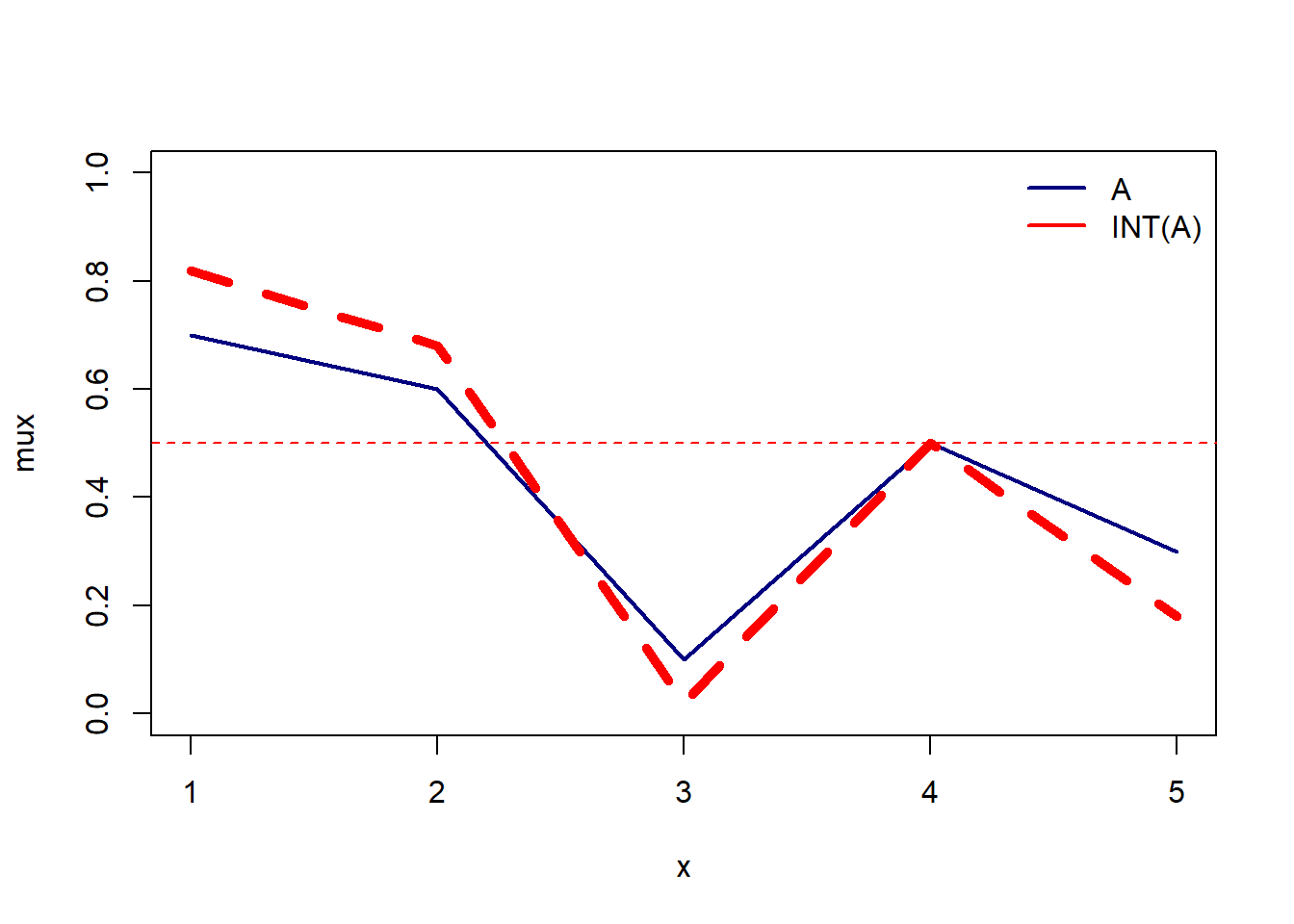
The contrast Intensification on a linguistic variable A is defined by INT(A) = $2A^{(2)}$ for $0 <= \mu_A(x) <= 0.5$ and $¬2(¬A)^{(2)}$ for $0.5 <= \mu_A(x) <= 1$.

Contrast Intensifier increases the values of $\mu_A(x)$ which are above 0.5 and reduces those below 0.5. Thus, it has the effect of reducing the fuzziness of the linguistic variable A.

Let’s take an discrete fuzzy set A = 0.7/1 + 0.6/2 + 0.1/3 + 0.5/4 + 0.3/5.

For x = 1, we have $¬2(¬A)^{(2)}$ = $1 - 2(1-0.7)^2$ = 0.82
For x = 3, we have $2A^{(2)}$ = $2*0.1^2$ = 0.02

We end up with, INT(A) = 0.82/1 + 0.68/2 + 0.02/3 + 0.5/4 + 0.18/5

A term set T(x) = $t_1(x),...,t_n(x)$ of a linguistic variable x defined on universe of discourse X is orthogonal if and only iff the sum of $\mu_{t_i}(x) = 1$ for all x $\in$ X where, $t_i(x)$ are convex and normal fuzzy sets.

Let’s consider three fuzzy sets :

A = 0.2/2 + 0.1/3 + 0.2/4 + 0.3/5
B = 0.6/1 + 0.6/2 + 0.7/4 + 0.7/5
C = 0.4/1 + 0.2/2 + 0.9/3 + 0.1/4

        1   2   3   4   5
A     0.0 0.2 0.1 0.2 0.3
B     0.6 0.6 0.0 0.7 0.7
C     0.4 0.2 0.9 0.1 0.0
Total 1.0 1.0 1.0 1.0 1.0

As the column totals i.e. sum of membership values of element is 1, we can say that the orthogonality condition holds for the terms set containing A, B, C.

A crucial application of the concept of a linguistic variable lies in the realm of approximate reasoning, a form of reasoning that is neither highly precise nor entirely imprecise. Consider the example where ‘x’ is small, and ‘x’ and ‘y’ are approximately equal, leading to the inference that ‘y’ is more or less equal.

In approximate reasoning, truth is treated as a linguistic variable, and its truth-values form a term-set, including terms like ‘true,’ ‘not true,’ ‘very true,’ ‘completely true,’ ‘more or less true,’ ‘fairly true,’ ‘essentially true,’ and so on.

Treating truth as a linguistic variable gives rise to fuzzy logic, which provides a more nuanced approximation to the logic involved in human decision processes compared to classical two-valued logic. In fuzzy logic, it becomes meaningful to assert statements that might be considered undefined or vague in classical logic.

For example, in fuzzy logic, the truth-value of ‘Liverpool is close to Manchester’ can be categorized as quite true, while the truth-value of ‘Leeds is close to Manchester’ may be fairly true. Consequently, the truth-value of ‘Leeds is more or less close to Liverpool’ is expressed as more or less true.

For further insights, the interested reader is encouraged to explore the research papers by Zadeh:

▪ Zadeh, L. A. The concept of a linguistic variable and its application to approximate reasoning—I.

▪ Zadeh, L. A. The concept of a linguistic variable and its application to approximate reasoning—II.

▪ Zadeh, L. A. The concept of a linguistic variable and its application to approximate reasoning—III.

There are some heuristics/ rule-of-thumb that can be applied to membership functions for linguistic variables:

The term set should span the universe of discourse.
The terms should not overlap too much. Overlap should normally be around 0.5 membership.
The number of terms should be small, usually odd number of terms (<= 7).
All terms should be normal and convex.

Fuzzy Inference System

A Fuzzy Inference System (FIS) is a key framework in fuzzy logic, utilized for deriving outputs from a set of inputs through fuzzy logic principles. The process involves several core components:

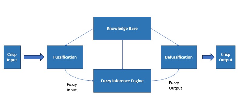
Fuzzification is the process of converting crisp input into a linguistic variable using membership functions stored in the knowledge base. For example, if the height of a person is 169 cm, it can be categorized under the fuzzy set ‘Medium.’
The Fuzzy Inference Engine conducts reasoning based on a collection of fuzzy if/then rules and available facts, facilitating the derivation of fuzzy conclusions.
The Knowledge Base acts as a central repository, storing the if/then rules and detailing the membership functions necessary for the system’s fuzzy logic operations.
Defuzzification,conversely, converts the fuzzy output generated by the system back into a precise, actionable value, bridging the gap between fuzzy logic processing and real-world application.

Fuzzy Reasoning

Fuzzy reasoning involves applying conditional IF-THEN rules that articulate relationships between inputs and outputs using linguistic variables or crisp values. In these rules, “x is A” forms the antecedent, setting the condition, while “y is B” comprises the consequence, specifying the outcome.

Let’s explore different rule structures in the following tabs.

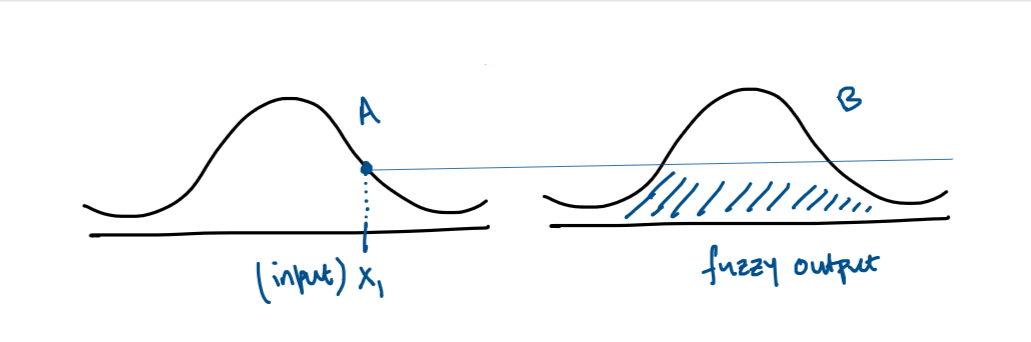
In scenarios where a single rule with a single antecedent is employed, such as “IF x is A THEN y is B,” the process begins with a crisp input (e.g., human height, ‘x1’) that is associated with a fuzzy set A. The essential step is to determine the input’s membership degree in fuzzy set A, which directly influences the resultant output in fuzzy set B.

The membership degree of ‘x1’ in set A is used to ascertain the corresponding output’s degree in set B, effectively generating a fuzzy output represented by a shaded area on the membership function of B. This fuzzy output encapsulates the rule’s effect given the specific input and serves as the basis for subsequent defuzzification, where it is converted back into a precise, crisp output value.

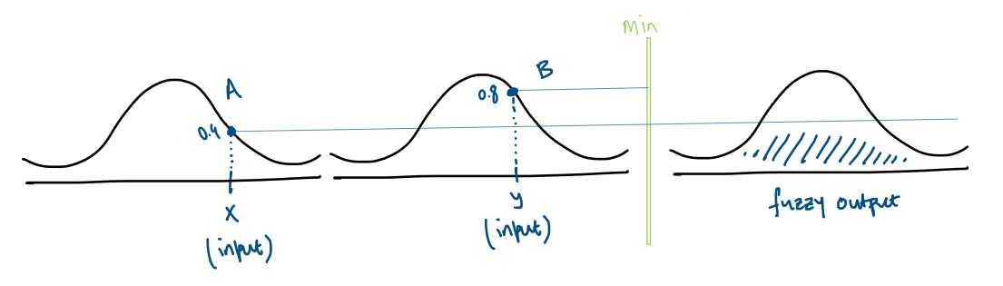
In situations involving a single rule with multiple antecedents, such as “IF x is A AND/OR y is B THEN z is C,” the rule structure introduces a choice between conjunction (AND) and disjunction (OR) to relate the antecedents. Utilizing AND suggests an intersection or minimum approach, indicating that the strength of the rule’s application is as strong as its weakest link. Conversely, OR implies a union or maximum, signifying that the strongest condition dictates the rule’s application.

Given two inputs, height $x_1$ associated with fuzzy set A and weight $y_1$ associated with fuzzy set B, we obtain two membership values, $w_1$ and $w_2$ , respectively. To determine the combined effect of these inputs on the consequent fuzzy set C, we apply a t-norm for AND (typically taking the minimum of $w_1$ and $w_2$ ) or a t-conorm for OR (taking the maximum). This operation yields the membership degree in the consequent fuzzy set C, represented as a shaded area, which captures the rule’s fuzzy output based on the specified logical relationship between the antecedents.

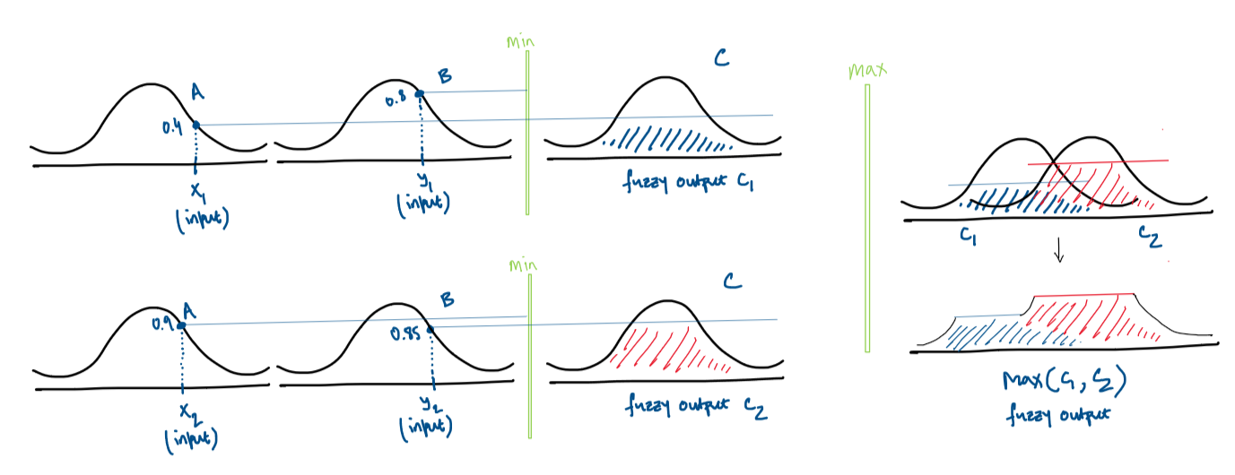
When handling multiple rules with multiple antecedents, we engage in a more complex fuzzy reasoning process that accommodates various scenarios simultaneously. Each rule, such as “IF x is $A_1$ AND/OR y is $B_1$ THEN z is $C_1$” and “IF x is $A_2$ AND/OR y is $B_2$ THEN z is $C_2$,” operates on its inputs to produce individual fuzzy outputs $C_1$ and $C_2$, respectively.

For each rule, the combination of antecedents through AND (intersection or minimum) or OR (union or maximum) determines the strength of the rule’s implication, reflected in the membership values of the consequent fuzzy sets $C_1$ and $C_2$,. After processing all rules individually, the next step is to aggregate these outputs to form a single composite fuzzy output.

This aggregation involves taking the maximum of the resulting fuzzy sets ($C_1$ and $C_2$, among others) using an S-norm operator, typically the maximum operator for simplicity and interpretability. This operation ensures that the final fuzzy output captures the strongest implications from all applicable rules, accommodating the contributions of each rule based on the inputs’ membership in their respective antecedent fuzzy sets.

In logic, an inference rule is a logical form comprising a function which takes premises, analyses their syntax and returns one or more conclusion.

Modus Ponens aka method of affirming is expressed as: if P (premise) And if P -> Q (premise), then Q (conclusion). Here, P -> Q is a conditional statement which reads: ‘if P is true, then Q is also true.’ For e.g., If it is raining (P), then I will stay inside (Q).

Modus Tollens aka method of denying in expressed as: if P -> Q, And if Not Q then not P. For e.g., If it is raining (P) then the ground is wet (Q). If the ground is not wet (not Q), it is not raining (not P).

The problem with these inference rules is that it does not capture the ambiguity in human language. For e.g., if there is light rain or drizzle, the ground may not be wet. Or, the ground could be wet due to other reasons. Modus Ponens is a valid and powerful deductive reasoning tool, but its effectiveness depends on the accuracy and clarity of the premises involved.

Fuzzy logic allows for more flexible interpretation of conditional statements, for e.g., If it rains heavily, then ground will be wet. If it rains lightly, then ground will be damp. If it does not rain, then the ground will be dry. These three statements enable us to capture varying degrees of truth & inherent vagueness in natural language.

Fuzzy Logic Models

Fuzzy Logic Models provide a structured framework for capturing and processing the ambiguity and uncertainty inherent in many real-world scenarios. These models leverage fuzzy logic principles to mimic human reasoning, enabling decision-making in complex environments where traditional binary logic falls short. Through the use of fuzzy sets, membership functions, and logical operations, these models offer a nuanced approach to handling imprecise information, making them invaluable across various fields and applications.

Named after its creator Lotfi Zadeh, the Mamdani Model proves particularly useful in scenarios involving human-like reasoning and linguistic expressions.

The Mamdani model employs a rule-based system to capture expert knowledge or human reasoning. Rules typically take the form of “IF-THEN” statements, where the antecedent (IF part) consists of fuzzy sets related to input variables, and the consequent (THEN part) involves fuzzy sets related to the output variable. Then we combine the antecedants using appropriate fuzzy operators (t-norm or s-norm), fire the rules at this combined strength to obtain the rule output based on the rule’s consequent. Then we aggregate the output for each rule using defuzzification methods.

The degree of truth of the antecedent of a rule is also known as the rule’s firing strength/degree.

The i-th rule $R_i$ = if $x_1$ is $A_i$, and $x_2$ is $B_i$ then $z$ is $C_i$, for $i=1,2,...n$
The Mamdani method uses minimum operator as fuzzy implication and the maximum operator for the composition.
The firing strength of the $i^{th}$ rule : $w_i$ = $min(\mu_{A_i}(x),\mu_{B_i}(x))$.

The Mamdani Fuzzy Model is widely used in various applications, such as control systems, decision support systems, and pattern recognition. It provides a way to model and implement human-like reasoning in systems that involve uncertainty or imprecision. Despite its popularity, it has some limitations, such as the need for expert knowledge to define fuzzy rules and the potential for complex rule bases in large systems.

Larsen in 1980 proposed the product implication. Unlike the Mamdani Model, which uses the minimum t-norm operator for ‘AND’ for aggression, Larsen uses the product t-norm operator to combine the results from different rules.

The firing strength of the $i^{th}$ rule : $w_i$ = $\mu_{A_i}(x)*\mu_{B_i}(x)$.
In the above example, the firing strength of rule 1 = 0.4*0.8 = 0.32 and of rule 2 = 0.9*0.85 = 0.765.

The TSK model was introduced by Takagi, Sugeno and Kang in 1985. It is quite similar to Mamdani Inference, but avoids the need for defuzzification. It uses antecedents in the same way as Mamdani, but polynomial functions for consequents. A typical fuzzy rule in TSK fuzzy model has the form :

IF $x$ is $A$ AND/OR $y$ is $B$ THEN $z$ = $f(x,y)$
where, $f(x,y)$ = $p_0$ + $p_1x$ + $p_2x^2$ + … + $p_mx^m$ + $q_1y$ + $q_2y^2$ + … + $q_my^m$.

Some points to be remembered :

Inputs are only crisp values.
When f(x,y) = constant, we have a Zero-order TSK Model.

Under the Mamdani system, the consequent is represented by a fuzzy set which needs defuzzification to yield crisp outputs. While under Zero-order TSK, the consequent is a constant value.

For example, If x1 is A, y1 is B then z is k = 8 & If x2 is A, y2 is B then z is k = 6.

The weighted average of the $k_i$ associated with each rule gives the overall output = $\sum_{i=0}^n w_i*k_i/\sum_{i=0}^n w_i$

In our example, $w_1 = min(0.4, 0.8)$, $w_2 = min(0.9, 0.85)$ and then $output = {0.4*8+6*0.85}/{0.4+0.85}= 6.64$.
When f(x,y) is a 1st order polynomial, we have a First-order TSK Model.

Advantage of Mamdani

Simple and Intuitive with a strong potential for XAI.
Well-suited for problems where linguistic rules are used to describe relationships between fuzzy sets of inputs and outputs. They are particularly effective when the system involves human expertise and the rules are expressed in a natural language form.

Advantage of Larsen

Suitable for cases where the consequence of a rule is computed by taking the product of the rule strength and the input fuzzy sets. They are simpler than Mamdani models and are often used in cases where simplicity and speed are crucial.

Advantage of TSK

Computationally efficient.
TSK works well with linear techniques e.g. PID Control
It is easier for optimization & adaptive techniques.
It has guaranteed continuous output surface.
It is effective in cases where a more mathematical and precise relationship between inputs and outputs is desired.
It does not require defuzzification.

The final choice of a fuzzy inference model depends on the use-case and how different models behave.

Defuzzification Methods

Defuzzification is a critical step in fuzzy logic systems, transforming fuzzy outputs back into crisp, actionable values. It bridges the gap between the nuanced reasoning of fuzzy logic and the precise requirements of real-world applications. The two primary approaches to defuzzification are numeric and linguistic defuzzification.

Numeric Defuzzification involves converting a fuzzy output into a specific numeric value, providing a definitive result based on the aggregated and processed fuzzy information. This approach is essential for applications requiring precise decision-making or control outputs. We will explore seven distinct methods of numeric defuzzification, each offering a different strategy for interpreting fuzzy outputs.

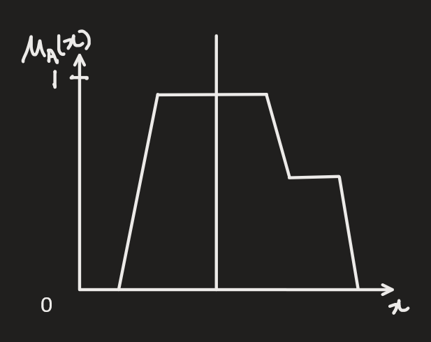
In this method, we simply take the value of z for which we attain the maximum membership. (here z is the variable representing our output fuzzy set).

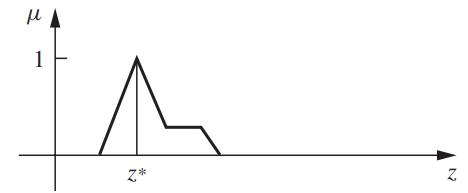
Centroid of Area or Mass is commonly used and provides a simple and intuitive solution. It calculates the center of mass of the fuzzy set.

Let us consider the following output fuzzy set A. The horizontal line reflects the centroid of this fuzzy set.

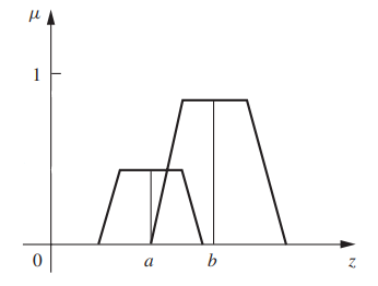
Centroid of Area (COA) = $\int x*\mu_A(x) dx / \int \mu_A(x)dx$

Here we deal with symmetric output membership functions. We take the centroid of each of these membership functions and then calculate a weighted sum of the two.

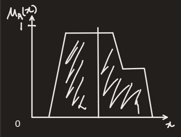
Let ‘a’ and ‘b’ be the respective centroids below and we assign weights $w_1$ and $w_2$ respectively. Then, $z_{wa} = (w_1*a + w_2*b) / (w_1 + w_2)$

Bisector of Area finds the x-coordinate where the area under the curve on either side is equal.

We first see the min-max values of x namely $\alpha$ and $\beta$. Then evaluate the below equation solving for $x_b$
$\int_{\alpha}^{x_b} \mu_A(x) dx$ = $\int_{x_b}^{\beta} \mu_A(x) dx$

These are three different methods where we take either Minimum, Average or Maximum of ‘x’ corresponding to maximum membership value.

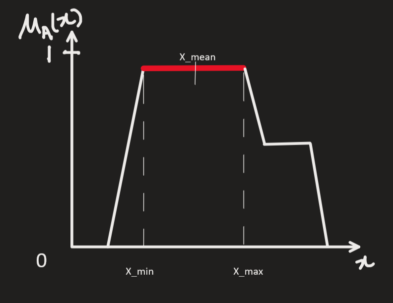
Say we attain the maximum membership of 1 for x between 5 to 7.
Smallest of Max = x_min = 5 (suppose)
Largest of Max = x_max = 7 (suppose)
Mean of Max = (5+7)/2 = 6

Centroid is suitable when the shape of the membership function is symmetric and has a clear center. It is among the most commonly used methods.
Bisector is suitable when the membership function is symmetric. However, it may not be ideal for skewed or asymmetric membership functions.
Smallest of Maximum is useful when we want to take a conservative approach as it ensures that the output is influenced by the least active rule.
Largest of Maximum comparatively a more aggressive approach giving more weight to the most active rule.
Mean of Maximum is a balance between the centroid and largest of maximum approaches. It useful in a lot of applications.

Linguistic Defuzzification contrasts with its numeric counterpart by translating fuzzy outputs into linguistic terms rather than precise numeric values. This approach leverages similarity and distance measures to determine the linguistic term that best represents the output set, offering an intuitive and qualitative way to interpret fuzzy logic conclusions.

For crisp sets, $J(A,B)$ = $|A∩B|$/$|A∪B|$
For fuzzy sets, $J(A,B)$ = $min(\mu_A(x),\mu_B(x))$/$max(\mu_A(x),\mu_B(x))$

Higher the value of $J(A,B)$, higher the similarity.

For example let’s consider two fuzzy sets A = {(1,1),(2,0.7),(3,0.3),(4,0.1),(5,0),(6,0)} and B = {(1,0),(2,0),(3,0),(4,0.5),(5,1),(6,0.3)}.

Numerator = min(1,0)+ min(0.7,0)+ min(0.3,0)+ min(0.1,0.5)+ min(0,1)+ min(0,0.3) = 0.1
Denominator = max(1,0)+ max(0.7,0)+ max(0.3,0)+ max(0.1,0.5)+ max(0,1)+ max(0,0.3) = 3.8
J(A, B) = 0.1/3.8 = 0.026

For crisp sets, $D(A,B)$ = $2*|A∩B|$/$|A|+|B|$
For Fuzzy sets, $D(A,B)$ = $2*\mu_A(x)*\mu_B(x)$/$(\mu_A(x)^2+\mu_B(x)^2)$

Dice Similarity is always more than equal to Jaccard Similarity.

Let’s continue with the same example above.

Numerator = 10+ 0.70+ 0.30+ 0.10.5+ 01+ 00.3 = 0.1
Denominator = 1+ 0.49+ 0.09+ 0.01+ 0.25+ 1+ 0.09 = 2.93
D(A,B) = 0.1/2.93 = 0.034

Jaccard vs. Dice Suitability : Jaccard considers intersection of sets in relation to the union thus providing a measure of how much two sets overlap. Dice on the other hand, takes account of both the size of intersection and the sizes of individual sets. Jaccard and Dice measures can be used in conjunction, providing complementary insights into the similarity between sets. The suitability of Jaccard and Dice measures depends on the problem domain and the nature of the sets being compared. It’s important to consider the characteristics of the data and the desired balance between commonality and distinctiveness.

Manhattan distance, also known as L1 Norm or city-block distance calculates the average absolute difference between elements. For fuzzy sets, $M(A,B)$ = 1/N * $\sum_{i=1}^N |\mu_A(x)-\mu_B( x)|$ where N is the number of discretisations on X-axis (i.e. count of vertical slices).
For M = 0, A & B overlap completely and are similar.
For M > 0, A & B overlap partially and are dissimilar.

Let’s take the same example.

M(A,B) = 1/6*(|1-0|+ |0.7-0|+ |0.3-0|+ |0.1-0.5|+ |0-1|+ |0-0.3|) = 3.7/6 = 0.62

Hausdorff distance calculates the distance between two sets based on alpha-cuts.
$H(A,B) = 1/M \sum_{i=1}^M max(|A_{\alpha_i}^- - B_{\alpha_i}^-|,|A_{\alpha_i}^+ - B_{\alpha_i}^+|)$
where, $A_{\alpha_i}^{-/+}$ is the left/right end-points of $\alpha$-cut of set A at $\alpha_i$ and M is the number of alpha-cuts considered.

Let’s consider $\alpha$ = {0, 0.2, 0.4, 0.6, 0.8} for the same example.

$A_\alpha$ = {[0.0,4.0],[0.3,3.5],[0.5,3],[1,2.5],[1.5,2]}
$B_\alpha$ = {[3.0,6.5],[3.5,6.2],[3.8,6],[4,5.7],[4.8,5]}
$H(A,B) = 1/5*[max(3,2.5)+max(3.2,2.7)+...max(3.3,3)]$ = 0.58

Manhattan vs. Hausdorff suitability : Manhattan and Hausdorff distances offer complementary perspectives on dissimilarity. While Manhattan distance focuses on the individual elements’ differences, Hausdorff distance considers the maximum difference between the sets. Hausdorff distance tends to be more sensitive to outliers or extreme values, so it might be more appropriate in situations where the focus is on capturing the maximum dissimilarity.

There are some desirable properties of similarity & distance measures:

Symmetry: $S(A,B) = S(B,A)$
Identity: $S(A,A) = 1$
Reflexive: $S(A,B) = 1$ iff A = B, and $D(A,B) = 0$ iff A = B
Transitive: A is subset of B is subset of C, then $S(A,B) >= S(A,C)$

If a Distance measure satisfies Triangle Inequality, it is called a Distance Metric.

Triangular Inequality: $D(A,B) <= D(A,C) + D(B,C)$

Generalizing Fuzzy Sets

Generalizing fuzzy sets to type-n fuzzy sets introduces an additional layer of sophistication and flexibility, allowing for a more nuanced handling of uncertainty. In this extended framework, the membership degrees of a type-n fuzzy set are defined in terms of fuzzy sets of type n-1, adding depth to the way uncertainty is modeled and processed.

Type-2 fuzzy set $A^\star =$ {(x,u), $\mu_A$(x,u) | $\forall x \in X, \forall$ u in $J_x \subset [0,1]$}.

The Type-2 fuzzy sets extend the concept of traditional type 1 fuzzy sets by introducing a higher level of uncertainty, where membership functions are themselves type-1 fuzzy sets.

The primary membership function, similar to type-1, maps the elements to a degree of membership between 0 and 1. The secondary membership function, represents the fuzziness in the membership grades. The combination of primary & secondary membership functions results in an area known as Footprint of Uncertainty (FOU), representing possible values of membership grades for each element.

Interval Type-2 fuzzy set $A*$ = {((x,u),1) | $\forall x \in X, \forall u \in J_x \subset [0,1]$}.

The Interval type-2 fuzzy sets have only one membership function, but with associated intervals. Thus, providing a simpler representation of uncertainty with a lower level of detail compared to type-2 fuzzy sets.

Intuitionistic fuzzy set $A*$ = {(x,$\mu_A(x)$,$\pi_A(x)$,$v_A(x)$) | $\forall x \in X$}, where $\mu_A(x) + \pi_A(x) + v_A(x) = 1$, 0 <= $\mu_A(x)$,$\pi_A(x)$,$v_A(x)$ <= 1.

Intuitionistic Fuzzy sets (IFS) are an extension of traditional fuzzy sets introduced by Krassimir Atanassov in the late 1980s. Here we model the degree of membership $\mu_A(x)$, non-membership $v_A(x)$ and a hesitancy index $\pi_A(x)$. The hesitation index represents the degree of hesitation or lack of confidence in the assignment of membership and non-membership values.

Non-Singleton Fuzzy Systems

Non-Singleton Fuzzy Logic Systems (NSFLSs) represent a significant advancement in dealing with the complexity and uncertainty inherent in real-world decision-making scenarios. Unlike traditional singleton fuzzy sets, NSFLSs employ non-singleton fuzzy sets to model inputs, allowing for a more nuanced representation of uncertainty.

In NSFLSs, two types of intervals, Epistemic Intervals (OR intervals) and Ontic Intervals (AND intervals), play a crucial role in capturing and quantifying uncertainty. Epistemic intervals reflect incomplete information about the actual value of an input, providing insights into the degree of uncertainty. On the other hand, Ontic intervals represent the actual distribution of values for an input, acknowledging the existence of multiple correct values.

Why use Non-Singleton Fuzzy Logic Systems?

NSFLS offer several advantages. They prevent unnecessary modifications to non-relevant aspects of the FLS when faced with input certainty, ensuring interpretability. NSFLS simplify the adaptation and design of FLS, making it easier to optimize the system as per evolving requirements. These systems enable accurate mapping of uncertainty models from inputs to antecedents, enhancing the reliability of the system in capturing and responding to uncertainty in input variables. Moreover, NSFLS demonstrate superior capabilities in handling uncertainty during inference, contributing to more robust decision-making in diverse uncertain scenarios.

There are two key challenges: (1) Fuzzification and (2) Composition.

The question here is how do we create fuzzy sets to represent our input and the uncertainty surrounding it.

Earlier we saw the use of fuzzy singleton where the input was represented as a fuzzy set with one element with membership equal to 1. But now, when we have an interval representing the input, we could use a triangular, gaussian or any other convex, non-convex fuzzy set.

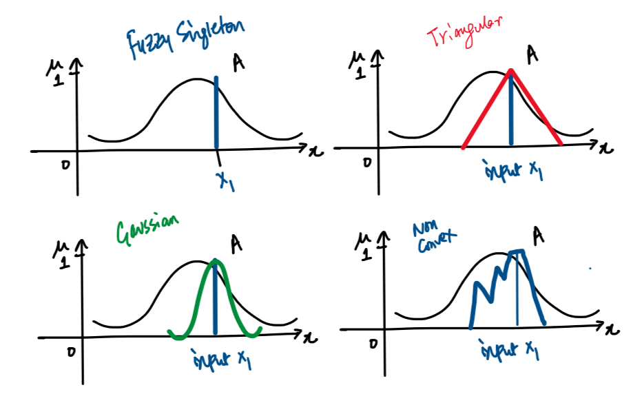
Now the input x1 is an interval represented by different distributions convex/ non-convex.

The question here is how do we map the input fuzzy set to the antecedent fuzzy set to generate the firing strength.

Method 1 - Standard Composition

Here, we simply take the maximum of intersection of input fuzzy set and the antecedent to give us the firing strength. This means that we consider the Intersection of A and I and then take maximum membership (equal to 0.7 in the figure below)

Method 2 - Centroid

Here, we calculate the centroid of the intersection of A and I. The firing strength is the membership value of the centroid.

Method 3 - Similarity-based

Here, we calculate the similarity index of A and I which gives us the firing strength. In the figure below we use Jaccard

Method 4 - Subset-hood

In this method, we calculate the subset-hood of A and I given by their intersection divided by the magnitude of input fuzzy set I.

$Subsethood = \int_x min(\mu_A(x), \mu_I(x)) dx / \int_x \mu_I(x) dx$

The Subset-hood method was proposed in this research paper: D. Pekaslan, J. M. Garibaldi and C. Wagner, “Exploring Subsethood to Determine Firing Strength in Non-Singleton Fuzzy Logic Systems,” FUZZ-IEEE, Rio de Janeiro, 2018, pp. 1-8.

The research shows how the subset-hood method performs better & more intuitively than standard, centroid and similarity-based methods under varying levels of noise.

Conclusion

This article is part of a comprehensive series on Fuzzy Logic and Systems using R, laying the groundwork for understanding advanced concepts and applications in this field.

For further exploration, you can access other articles in this series:

The work in this article is inspired by the teachings of my Professors at the University of Nottingham. Their guidance and expertise have greatly influenced the content and direction of these articles. For further insights into their research and contributions, you can visit their University of Nottingham profiles:

These articles aim to delve deeper into Fuzzy Logic concepts and their practical implementations, building upon the foundation laid by our esteemed professors. Stay tuned for more valuable insights and applications in this exciting field.